Simulation Monte Carlo

Your revenue forecast passed backtesting, the dashboard looked stable, and the pipeline shipped on schedule. Then production data arrived late, an upstream field carried unexpected errors, and several dependent transformations amplified the discrepancy. By the time the business team asked why actual revenue had diverged, deterministic tests had little to say because they had tested fixed inputs, not the uncertainty surrounding the pipeline.

Simulation Monte Carlo gives data teams a practical way to model that uncertainty. Instead of treating every input as a single value, you represent uncertain inputs as distributions, run the pipeline logic repeatedly, and inspect the resulting range of outcomes. The method helps teams reason about data quality thresholds, KPI volatility, pipeline capacity, and downstream risk without pretending that production behaves like a clean test fixture.

Table of Contents

• Why Data Teams Need Monte Carlo Simulation

• Understanding the Core Mechanics

  • Sampling inputs

  • Aggregating outcomes

• Algorithms and Sampling Methods Explained

  • Choosing a method

• How Many Simulations Are Enough

  • Use a stopping rule

• Real-World Applications in Data Quality and Monitoring

  • Data quality scenarios

  • Connecting results to observability

• Implementation Patterns and Performance Trade-Offs

• Common Pitfalls and How to Avoid Them

• Integrating Monte Carlo Into Your Data Platform

  • Choose the execution path

  • Roll out in phases

Why Data Teams Need Monte Carlo Simulation

A modern data platform rarely produces a metric through one isolated calculation. A revenue figure may depend on event ingestion, identity resolution, currency conversion, late-arriving records, deduplication, business rules, and several warehouse transformations. Each dependency can introduce uncertainty, and the combined effect may be nonlinear.

A point estimate hides that structure. If a team tests a conversion rate with one expected input, it can verify whether the formula works for that input, but it can't answer how the output changes when event counts fluctuate, attribution is incomplete, or source data arrives outside its expected window. Deterministic testing validates a path. Monte Carlo simulation examines a distribution of paths.

That distinction matters for operational decisions:

• Data quality SLAs: Estimate how often uncertain source defects could push a downstream table beyond an acceptable threshold.

• Business monitoring: Separate ordinary KPI variation from changes that deserve investigation.

• Capacity planning: Explore workload combinations instead of sizing infrastructure against a single average.

• Pipeline resilience: Identify which upstream assumptions create the widest range of downstream outcomes.

A data team can pair probabilistic analysis with established data quality practices. Deterministic checks still matter for schema, nullability, referential integrity, and explicit business rules. Monte Carlo adds a different layer, one that asks whether plausible variation in those inputs could create an operational incident.

Practical rule: Use Monte Carlo to quantify uncertainty around a decision, not to excuse weak validation. A simulation can't repair an incorrect transformation or an unobserved source dependency.

The value appears when teams stop asking only, “Did this run pass?” and start asking, “Given what we know about this system, how likely is the result to remain within bounds?” That question is much closer to the nature of enterprise data operations.

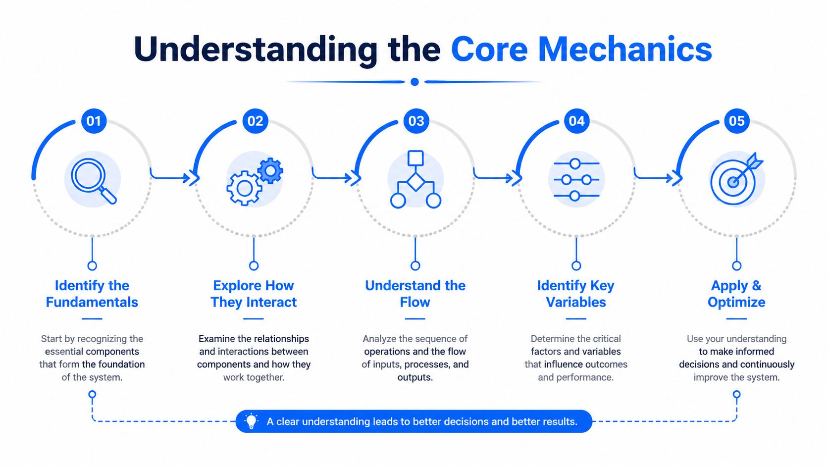
Understanding the Core Mechanics

Start with a pipeline as a function:

output = pipeline(input_1, input_2, input_3)

In ordinary testing, each input receives a fixed value. In Monte Carlo work, each uncertain input receives a probability distribution. The pipeline then runs repeatedly with sampled values, producing an output distribution rather than a single answer.

Sampling inputs

Random sampling is the atomic operation. A random-number generator selects a plausible value from each input distribution, and the model processes that combination as one possible system state.

The distribution should reflect the behavior of the input:

• Normal distributions can represent measurement errors when values cluster around an average.

• Poisson distributions are useful for event counts, such as arrivals within a defined observation window.

• Uniform distributions fit bounded uncertainty when there is no defensible reason to favor one value over another.

• Empirical distributions are often preferable when historical observations show skew, multimodality, or unusual tails.

Historical data can inform the distribution, while domain knowledge can fill gaps where observations are sparse. The important point is not to select a familiar distribution by habit. The shape of the input distribution directly influences the output.

For a data engineer, the process resembles generating synthetic test data at scale. Each iteration creates a coherent set of uncertain inputs, executes the transformation logic, and stores or aggregates the result. The final output behaves like a materialized view over many plausible operating conditions.

Aggregating outcomes

The simulation loop has three practical stages:

1. Define distributions. Use historical observations, fitted parameters, or documented domain assumptions.

2. Sample and execute. Draw values and run the same model logic for each iteration.

3. Aggregate results. Calculate ranges, percentiles, confidence intervals, and threshold probabilities.

The Law of Large Numbers explains why repeated sampling becomes useful. As the number of independent samples grows, summary statistics tend to converge toward the underlying distribution. That convergence doesn't make the model true, but it reduces uncertainty caused by random sampling.

The model still depends on the quality of its inputs and implementation. Teams looking for a deeper explanation of how distributions describe observed values can consult this guide to the distribution of data.

Algorithms and Sampling Methods Explained

Simple random sampling should be the baseline, not a permanent default. It works well when inputs are reasonably independent, the dimensionality is manageable, and the business question concerns central behavior rather than a thin tail. Its main advantage is operational simplicity, which makes it easier to test, explain, and reproduce.

The method becomes less attractive when the simulation must cover heterogeneous populations or rare outcomes. Sampling design should follow the question, the dependency structure, and the compute budget.

Choosing a method

Stratified sampling divides the population into meaningful groups and samples within each group. This prevents a large segment from dominating the result while a smaller but operationally important segment receives little representation. For example, a data quality model can preserve coverage across customer tiers or geographic regions rather than treating all records as interchangeable.

Latin Hypercube Sampling spreads samples across each input dimension. It can improve coverage when a pipeline has many uncertain variables and each run is expensive. The overhead is justified when input dimensionality makes simple random draws leave large parts of the space unexplored. It isn't necessary for a small model where each run is cheap and the output is stable.

Importance sampling changes the sampling emphasis toward outcomes that matter but occur infrequently. It fits corruption detection, severe SLA breaches, or other tail questions, provided the weighting scheme is carefully validated. Without that validation, the method can create a convincing but biased estimate.

Markov Chain Monte Carlo is appropriate when variables have dependencies that prevent reliable independent sampling. It offers flexibility for complex joint distributions, but teams must monitor chain behavior and mixing. If independent or stratified samples already answer the question, that complexity isn't worth carrying into production.

A useful selection rule is straightforward: start simple, move to variance reduction when compute is the bottleneck, and use dependency-aware methods when independence is demonstrably false. Guidance on applying statistical methods for data analysis can help teams align the method with the data problem rather than choosing an algorithm because it sounds advanced.

How Many Simulations Are Enough

A fixed instruction such as “run 10,000 simulations” is a poor production policy. The required replication count depends on output variance, the precision decision-makers need, and the cost of each model execution. A stable, low-variance metric may need far fewer runs than a volatile tail estimate. A complicated model can remain unreliable even after many iterations.

A 2022 review found that modellers often choose replication counts without scientific justification. That can produce too few runs, leaving the sample mean unrepresentative, or too many, wasting compute that could support better model analysis. The same review is discussed in this source on replication and stopping practice.

Use a stopping rule

Define a measurable stopping condition before execution starts. Useful criteria include:

• Standard error threshold: Stop when the estimated standard error of the target metric falls below the decision tolerance.

• Confidence interval width: Stop when the interval around the estimate is narrow enough for the operational use case.

• Coefficient of variation: Track relative dispersion and stop when it stabilizes within an agreed range.

• Quantile stability: For tail estimates, compare the target percentile across checkpoints instead of monitoring only the mean.

Check convergence after each fixed batch, not after every run. A scheduler can append a batch, calculate diagnostics, and terminate once the rule is satisfied. This pattern works for warehouse SQL jobs, Python workers, and distributed execution. Set the checkpoint size with transaction overhead and cluster startup costs in mind.

The stopping rule belongs to the decision. A data quality alert may tolerate a wider interval because it triggers investigation rather than an irreversible financial decision. A risk calculation may require tighter bounds and stronger validation. Teams documenting data reliability measurement should record the tolerance, checkpoint schedule, and metric used to stop.

Do not add iterations automatically when convergence fails. Check the input distributions, correlations, implementation, and random-number generation first. More samples reduce sampling noise, but they do not correct a flawed model.

Monte Carlo uncertainty reporting remains a weakness in simulation practice. A methodological review identified failure to report it as one of the main shortcomings in simulation studies. A 2024 paper argued that poor design and reporting can enable spurious superiority claims in comparative simulations. Convergence diagnostics and transparent reporting therefore belong in the production workflow, alongside the model code and pipeline metadata.

Real-World Applications in Data Quality and Monitoring

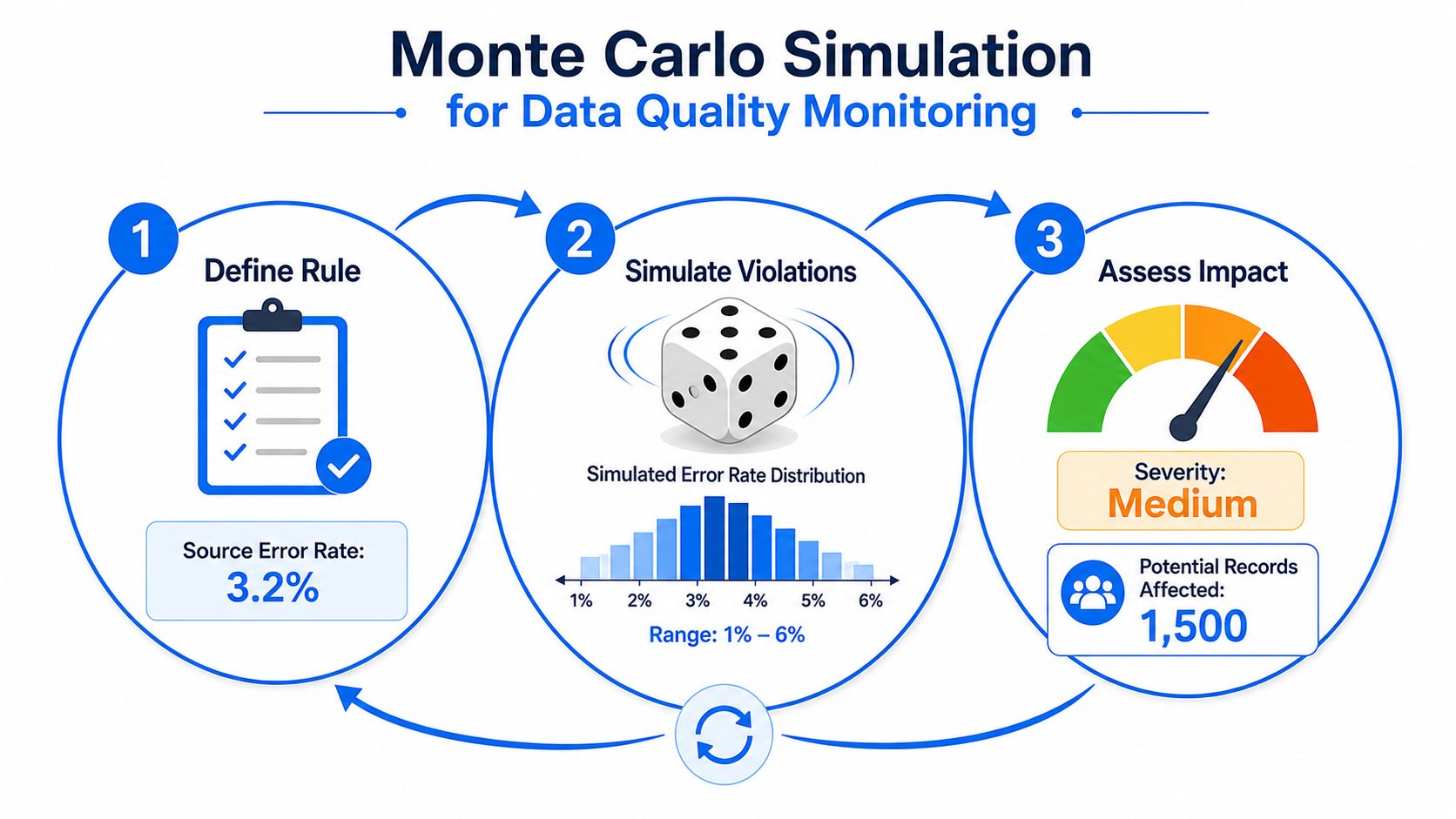
Monte Carlo becomes operationally useful when its output feeds an existing monitoring decision. Consider a source table with an uncertain defect rate. The team can sample plausible defect rates, inject violations into a representative dataset, run downstream rules, and calculate the probability that affected records exceed an agreed threshold.

That calculation doesn't replace a null check or a uniqueness test. It answers a different question: given uncertainty in the source, how exposed is the downstream system?

Data quality scenarios

A practical workflow can model:

• Rule violations: Estimate the range of records that could fail a validation rule under changing source conditions.

• Late arrivals: Propagate delivery-time uncertainty into the completeness of a reporting window.

• KPI uncertainty: Build confidence bands around derived metrics whose inputs are measured imperfectly.

• Anomalies: Compare an observed result with a simulated distribution and flag values in extreme tails.

• Capacity demand: Generate workload combinations to evaluate warehouse or orchestration pressure.

For a SQL-oriented implementation, a warehouse table can hold simulation identifiers, sampled parameters, and output metrics. A simplified pattern looks like this:

select
  simulation_id,
  uniform_sample as assumed_error_rate,
  source_records,
  round(source_records * uniform_sample) as simulated_violations,
  case
    when source_records * uniform_sample > threshold then true
    else false
  end as breaches_threshold
from simulation_inputs;

select
  simulation_id,
  uniform_sample as assumed_error_rate,
  source_records,
  round(source_records * uniform_sample) as simulated_violations,
  case
    when source_records * uniform_sample > threshold then true
    else false
  end as breaches_threshold
from simulation_inputs;

select
  simulation_id,
  uniform_sample as assumed_error_rate,
  source_records,
  round(source_records * uniform_sample) as simulated_violations,
  case
    when source_records * uniform_sample > threshold then true
    else false
  end as breaches_threshold
from simulation_inputs;

The production version should use the warehouse's supported random functions, persist the seed or run configuration, and keep the threshold in a governed parameter table. The key design choice is to make the result queryable by the same dashboards and alerting jobs that consume deterministic checks.

Connecting results to observability

Simulation outputs should become first-class observability signals. Store the run timestamp, model version, input assumptions, convergence diagnostics, relevant percentiles, and the probability of crossing each alert threshold. Dashboards can show the expected range, while incident systems can route only materially unusual results to the owning team.

Teams working on Monte Carlo simulations for data anomaly detection can use this pattern to complement baseline monitoring. An observed metric outside the simulated range isn't automatically proof of a data defect, but it provides a disciplined trigger for checking source freshness, schema changes, pipeline latency, and business events.

Implementation Patterns and Performance Trade-Offs

Execution location determines more than speed. It affects data movement, library access, security review, cost visibility, reproducibility, and who can operate the job after it reaches production.

In-database execution keeps data close to the transformations. SQL can sample inputs, join simulation parameters, execute warehouse-native logic, and persist results without exporting sensitive records. This pattern works well when the model mirrors existing transformations and the warehouse can parallelize the workload.

Its limits appear when the team needs advanced samplers, custom probability distributions, iterative chains, or specialized diagnostics. Procedural SQL can support more logic, but complexity may become difficult to test and expensive to run.

External Python, R, or Spark workers offer a broader ecosystem. NumPy, SciPy, PyMC, and distributed frameworks can simplify advanced sampling and model diagnostics. The trade-off is serialization overhead, credential management, network movement, separate deployment pipelines, and additional governance work.

Precompute when inputs change on a schedule and consumers need predictable latency. Run on demand when analysts are exploring assumptions or responding to an incident. Cache results when the input snapshot, parameter set, model version, and random seed are unchanged. A cache without those keys can return a fast but misleading answer.

Reproducibility requires deliberate controls. Seed random-number generators, version model code and parameters, record the source snapshot, and retain audit metadata. Regulated environments may also need approval records and a clear distinction between exploratory and production runs.

Common Pitfalls and How to Avoid Them

Monte Carlo models often fail without warning. The output distribution looks polished, the percentile chart renders correctly, and the underlying assumptions remain unsuitable for the data.

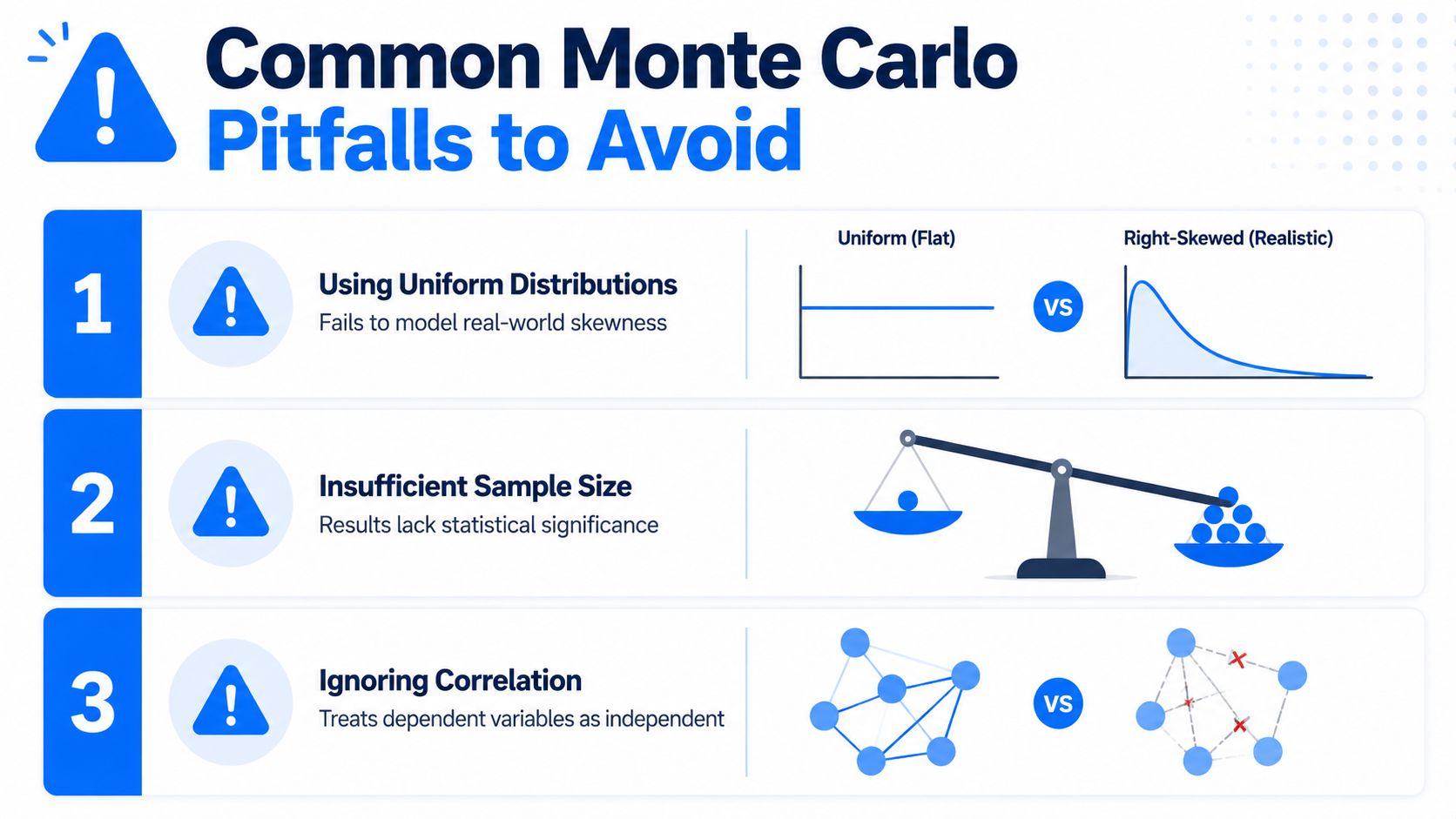
The first mistake is selecting a uniform distribution because a minimum and maximum are easy to provide. Real operational data may be skewed, clustered, truncated, or affected by seasonality. Fit candidate distributions against historical observations, inspect residual behavior, and use an empirical distribution when no simple family represents the data adequately.

The second is treating dependent inputs as independent. A late source load may coincide with lower record completeness, while a high workload may increase processing latency. If the model samples those variables separately, it can create combinations that never occur or miss combinations that matter.

Model relationships, not just columns. A plausible marginal distribution can still produce an implausible system when the correlation structure is wrong.

The third pitfall is confusing a probabilistic range with a deterministic forecast. A simulated percentile isn't a promise, and a tail observation from a weakly sampled distribution shouldn't drive a major decision without validation.

Use a compact validation routine:

• Distribution fit: Apply a Kolmogorov-Smirnov test where its assumptions fit the data, then inspect the visual fit rather than accepting a test result mechanically.

• Sensitivity analysis: Identify which inputs explain output variance and focus data collection or controls there.

• Seed checks: Run the same configuration with a documented seed in CI/CD and verify that differences stay within an accepted tolerance.

• Stress scenarios: Add deliberately adverse but plausible combinations to test whether the model behaves sensibly outside its central range.

• Output review: Compare simulated behavior with historical outcomes and investigate systematic disagreement.

Variance reduction can improve compute efficiency, but it shouldn't be added as decoration. Use it when diagnostics show that simple sampling spends too much effort in irrelevant regions or fails to resolve the decision boundary.

Integrating Monte Carlo Into Your Data Platform

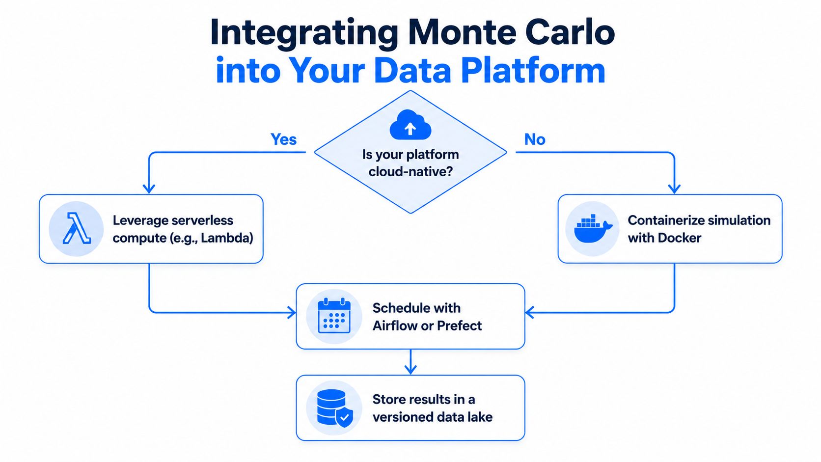
A useful architecture starts with the existing data product, not the simulation library. Keep deterministic validation close to the data, then add simulation jobs where uncertainty changes the operational decision.

Choose the execution path

Use a dbt macro or warehouse SQL when the model uses relational transformations, the data must remain in place, and scheduled results are sufficient. Use a dedicated Python worker orchestrated by Airflow or Dagster when the simulation needs advanced sampling, probabilistic programming, or richer diagnostics.

Whichever path you choose, persist:

• Input snapshot identifiers: So the team can reconstruct what the model consumed.

• Parameter versions: So distribution assumptions don't change invisibly.

• Model and code versions: So output changes can be attributed.

• Convergence metadata: So consumers can distinguish a completed run from an unstable one.

• Decision thresholds: So alert behavior remains auditable.

Cache results for unchanged inputs and parameters. Invalidate the cache when source data, model code, distribution parameters, or thresholds change. Observability systems can consume the resulting metrics alongside freshness, schema, validation, and anomaly signals.

Roll out in phases

Begin with historical backtesting. Compare simulated ranges with known pipeline outcomes and document where the model misses. Next, schedule the simulation beside existing data quality jobs and send its outputs to dashboards, alert routing, and incident records.

Only after those stages are stable should the team consider incident-triggered or near-real-time execution. At that point, success means more than producing a distribution. The workflow should identify the affected datasets, explain which assumptions drove the alert, preserve the run context, and give an owner enough evidence to act.

digna offers in-database data quality validation, anomaly detection, timeliness monitoring, schema tracking, and business metric observability inside a customer's environment. Visit digna to evaluate how its observability capabilities can complement a production simulation monte carlo workflow, then start with one monitored dataset, one governed model, and a stopping rule you can defend.