Monte Carlo Risk Assessment: A Practical Guide
|
7
min read
Monday morning starts with a dashboard anomaly nobody can explain. Revenue appears to have jumped sharply, finance calls an urgent review, and engineers begin tracing logs across ingestion, transformation, and reporting jobs. By midday, the team discovers that a delayed upstream pipeline caused Saturday's transactions to be counted twice. The alert worked, but the response still lacked the number leadership needed: how likely was the error, how large could the exposure become, and which decision should change because of it?
That distinction defines Monte Carlo risk assessment. A data-quality alert tells you that something has moved outside an expected pattern. A simulation estimates the range of business outcomes that could follow, using uncertainty from pipeline latency, record volumes, validation failures, and downstream use. The method connects “the data may be wrong” with “this is the probability and impact we should plan against.”
Table of Contents
When the Real Risk Is the Data Behind the Dashboard
Alerts describe events, not exposure
From broken data to a defensible decision
The Core Idea Behind Monte Carlo Risk Assessment
Translate the question into a simulation
The three ingredients
The Five Stages of a Trustworthy Simulation Workflow
Stage one, frame the decision
Stage two, source the uncertainty
Stage three, build the propagation model
Stage four, run and preserve
Stage five, communicate the distribution
Building the Model Inside Your Data Platform
Turn telemetry into inputs
Propagate uncertainty through business logic
Reading the Outputs Like a Risk Analyst
Three artifacts deserve attention
Report the tail, not just the center
Pitfalls That Make Simulations Non-Auditable
Independence is often the convenient fiction
The tail disappears when the shape is wrong
Two Real-World Examples From Finance and Data Quality
Data quality has the same structure
Observability becomes the sampling layer
Choosing When Monte Carlo Is the Right Tool
When the Real Risk Is the Data Behind the Dashboard
At 8 a.m., the CFO sees an unexpected revenue surge and asks finance to validate it before the executive meeting. Analysts compare the dashboard with the warehouse, engineers inspect orchestration logs, and data owners check whether the source system changed. Each person has part of the story, but nobody can immediately quantify the exposure.
By late morning, the root cause is clear. A delayed upstream load duplicated Saturday's transactions. The dashboard wasn't merely showing an unusual value. It was presenting a business decision on top of a compromised data path.

Alerts describe events, not exposure
The team had monitoring. It could identify a delayed job, a row-count change, or an unexpected metric. What it couldn't answer was how the failure might propagate:
Duration: How long could the pipeline remain incorrect before detection?
Scope: Which tables, reports, and models could inherit the defect?
Business effect: Which revenue, risk, or compliance decisions could be affected?
Response: Should finance pause reporting, apply a correction, or continue with a documented caveat?
That's the deeper failure. Alerts are observations. Risk assessment is decision support. A data observability program can help teams understand the health and behavior of datasets, as described in digna's overview of data observability, but the next step is translating those observations into probable outcomes.
From broken data to a defensible decision
A Monte Carlo model can sample plausible combinations of delivery delay, duplicate volume, correction time, and dashboard usage. Each run represents one possible operational scenario. The output becomes a distribution of exposure rather than a single guess.
That shift matters during incident response and routine governance alike. Instead of telling leadership that “the revenue table is unreliable,” the data team can present a range, identify the drivers of uncertainty, and state which threshold is likely to be exceeded. The rest of this guide turns that bridge into a reusable workflow for warehouse and pipeline teams, with auditability treated as part of the model rather than an afterthought.
The Core Idea Behind Monte Carlo Risk Assessment
A Friday revenue dashboard is due, but its source table sometimes arrives late. One run may show a normal refresh, while another includes an upstream delay, a failed job, and a slow repair. The question is not whether one specific outcome will occur. It is how often plausible combinations of events could push freshness or business exposure beyond an acceptable threshold.
A coin toss provides a simple starting point. With ten flips, you can observe several heads and tails, yet the balance remains uncertain. That small sample gives one outcome, not a dependable view of the process.
Repeat the experiment across ten thousand flips, and the results support probability statements. You can examine the distribution, compare its center with its extremes, and estimate how often it crosses a chosen threshold. The computer is not guessing. Repeated trials expose the shape of uncertainty.

Translate the question into a simulation
Suppose a data platform engineer asks, “How often will this table be stale by more than thirty minutes on a given Friday?” Several uncertain inputs affect the answer:
The source's normal arrival pattern.
Delay from upstream dependencies.
The chance that a job fails or retries.
The time needed to detect and repair the issue.
The business impact of stale data during that reporting cycle.
A deterministic calculation assigns one latency value to each input. A Monte Carlo simulation samples values from probability distributions, passes them through a system model, and records the resulting freshness or financial outcome. Repeating that process turns an observability signal into quantified business risk. A platform such as digna can connect this reasoning to Monte Carlo methods for better data observability, so simulation results can be reviewed as evidence rather than treated as an opaque forecast.
Practical rule: The value comes from structured exploration of uncertainty, not randomness alone.
The three ingredients
Every credible simulation has three components.
A system model: This maps inputs to an outcome. It can be a formula, directed acyclic graph, SQL logic, or Python simulation harness.
Input distributions: Each uncertain variable needs a defensible range and shape. Historical telemetry, service commitments, and documented expert judgment can inform those distributions.
Enough iterations: The model runs repeatedly until its output is stable enough for the decision. More runs clarify the simulated distribution, but they cannot correct weak assumptions.
Monte Carlo methods have a long history. Early probabilistic ideas include Buffon's needle experiment. Modern risk applications developed through wartime scientific computing and work associated with the Manhattan Project. Stanisław Ulam conceived the approach at Los Alamos in 1946, John von Neumann helped develop it in 1947, and the method was first used to calculate neutron diffusion paths for the hydrogen bomb, as documented in this historical account of Monte Carlo methods. Repeated sampling later made difficult quantities more approachable in fields such as nuclear safety analysis and financial volatility modeling.
For a data team, the translation is direct: define what can vary, describe how it varies, pass those inputs through the business logic, and inspect the resulting distribution. Store the assumptions, sampled inputs, model version, and outcome so the simulation can support audit and governance, not merely produce a warning.
The Five Stages of a Trustworthy Simulation Workflow
A histogram is only an intermediate result. A governance-ready workflow lets another engineer, auditor, or risk committee understand how the result was produced and replay it from the recorded evidence.
Stage one, frame the decision
Start with a business question rather than a technical symptom. “What is the probability that reported revenue exceeds the correction threshold?” identifies an outcome, threshold, and decision owner. “How unstable is the transaction table?” describes a condition but does not define an action.
Record the reporting period, affected datasets, downstream consumers, acceptable uncertainty, and response for each risk band before selecting a distribution. This scope keeps the simulation tied to a decision instead of turning into an open-ended data exercise.
Stage two, source the uncertainty
List every variable that can change the outcome and connect it to evidence. Historical arrival telemetry can describe freshness behavior. Vendor commitments can provide an external prior for service delays. Validation results can show how often invalid records occur and how large their effect may be.
Document the reason for each distribution choice. A parameter without its source leaves reviewers unable to separate measured behavior from an analyst's judgment. That distinction matters when assumptions change or a result must be defended later.
Stage three, build the propagation model
The model may be a formula, dependency graph, or simulation harness. It should expose the path from each sampled input to the business outcome. If delayed data changes a dashboard metric, the logic should identify the affected records, calculate the metric change, and show where downstream weighting enters.
Stage four, run and preserve
Run enough iterations for the selected output to stabilize. Capture the random seed, model version, library versions, input snapshot, and raw draws. A final percentile without this record cannot support reliable replay or effective debugging.
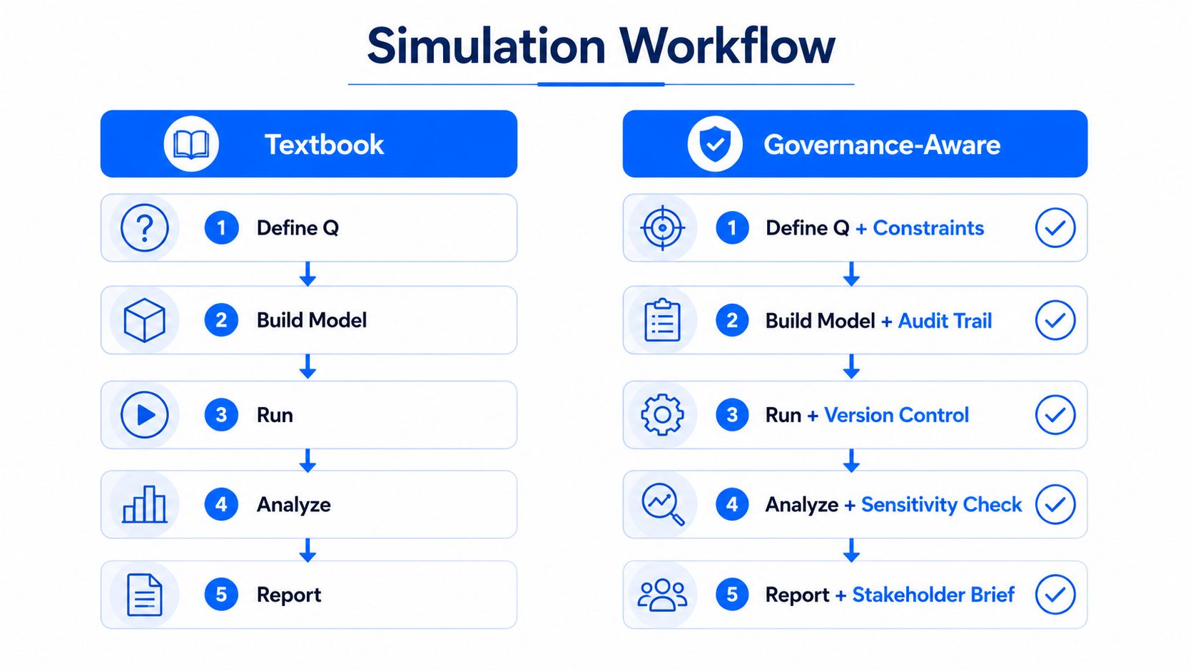
Stage five, communicate the distribution
Leadership usually needs the plausible interval, relevant tail, main drivers, and action associated with the result, rather than every simulated row. Present percentile bands and sensitivity evidence, while retaining the complete model record for review. Tools such as digna can turn repeated simulations into auditable, governance-ready evidence about the business risk created by bad data.
Governance provides the evidence trail that makes a simulated risk number defensible during regulatory review or executive review, especially when financial consequences require defensible reasoning.
Building the Model Inside Your Data Platform
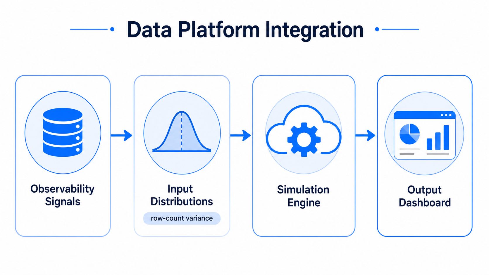
A warehouse-native model starts with observability signals that already describe how the data product behaves. Instead of exporting metrics into a side spreadsheet, the platform can assemble distributions, execute the simulation, and store outcomes alongside the source metadata.
Turn telemetry into inputs
Different signals describe different kinds of uncertainty:
Row-count variation can inform a count model, such as a Poisson-style model for event arrivals or a normal approximation when the process is sufficiently stable.
Null-rate drift can be represented with a beta distribution because rates are bounded and may change asymmetrically.
Freshness lag can use a shifted lognormal shape when delays remain nonnegative and occasional long delays matter.
Schema changes and validation failures can feed scenario variables that alter the affected population or invalidate a downstream calculation.
These choices aren't automatic truths. The team should compare candidate distributions with historical behavior, inspect tails, and record the rationale. A distribution that looks convenient but misrepresents the source process can create false confidence.
Propagate uncertainty through business logic
Consider a revenue model expressed as:
revenue = transactions × price × (1 - refund_rate)
The simulation samples transaction volume, price, and refund rate for each run. It then applies the formula and stores the resulting revenue outcome in a results table. A warehouse implementation might use SQL for aggregation and a lightweight Python job for distribution sampling, while a more complex model could use a dedicated simulation engine.
The operational detail matters. Store the source snapshot, feature definitions, model code version, random seed, distribution parameters, and dependency versions with every run. If a pipeline changes later, reviewers should be able to distinguish a new risk state from a change in the model itself.
An in-database approach also reduces unnecessary movement of sensitive data. digna's in-database data quality approach describes a pattern where metrics and analysis execute within the customer's database environment. In a Monte Carlo workflow, anomaly scores, timeliness signals, validation outcomes, and schema differences can become versioned inputs rather than disconnected alerts.
Reading the Outputs Like a Risk Analyst
A histogram is evidence, not a conclusion. The analyst's job is to identify the interval, the tail, and the inputs that create the spread.
Three artifacts deserve attention
Percentile bands bound the plausible range of outcomes. They let you state how much of the simulated probability mass falls below or above a threshold. A finance partner can act on an interval more effectively than on an unexplained average.
Fan charts show how uncertainty widens across time or successive forecast points. In a data platform, they can illustrate the projected range of freshness, accumulated reporting exposure, or a metric under repeated dependency delays.
Tornado plots rank input variables by their contribution to outcome variance. They're useful because they redirect remediation toward the uncertainty that matters most. If freshness lag dominates the spread, tuning a low-impact validation rule won't materially change the risk profile.
Report the tail, not just the center
A skewed distribution can make the mean a poor headline number. The average may sit comfortably below a threshold while a meaningful tail extends into unacceptable exposure. For risk reporting, a tail percentile is often more auditable because it states the boundary the organization is choosing to manage.
A properly qualified statement might look like this: “Ninety-five percent of runs land between 1.8 million and 2.4 million, while the fifth-percentile revenue tail is 1.4 million.” Those values are an illustrative reporting format, not a universal result. Your model must supply the actual interval and document the assumptions behind it.
The distribution of data provides the foundation for interpreting these shapes. Confidence belongs to the interval or percentile statement, not to a single point estimate. Always pair the headline with the model scope, input snapshot, and sensitivity result.
Pitfalls That Make Simulations Non-Auditable
A simulation can produce a polished chart while encoding weak assumptions. The most dangerous failures are quiet ones, because the output looks more rigorous than the process that generated it.
Independence is often the convenient fiction
Treating inputs as independent is easy to implement, but pipeline failures often share causes. A source delay can increase freshness lag, reduce available records, and trigger downstream retries at the same time. A 2025 project-risk study found that adding probabilistic dependencies and temporal cascade effects produced significantly higher contingency requirements than classical approaches, while a 2022 systematic review emphasized dependence modeling, tail-aware fitting, and transparent validation in this review of project-risk methods.
Use correlation matrices or shared latent risk drivers where the evidence supports them. Then test whether simulated co-movement resembles observed behavior.
The tail disappears when the shape is wrong
A normal distribution can understate rare but consequential delays or losses when the underlying process is heavy-tailed. Inspect historical extremes, test alternative distributions, and run explicit stress scenarios for risks that the main model may not represent well.
Other guardrails belong in the run metadata:
Seed logging: Preserve the random seed so an approved run can be replayed.
Snapshot pinning: Tie input parameters to a specific data snapshot so source drift doesn't rewrite history.
Convergence checks: Compare key outputs across additional runs or seeds and record the stability decision.
Backtesting: Compare simulated ranges with later observed outcomes and revise the model when it consistently misses.
Formula review: Validate business constraints, exclusions, caps, and conditional paths instead of assuming a simplified equation is sufficient.
digna's explanation of data provenance and data lineage is useful context for separating where a value came from from how it moved through the platform. A trustworthy simulation needs both.
Two Real-World Examples From Finance and Data Quality
Finance offers a familiar application. A portfolio risk team can simulate correlated daily returns for equities and interest rates, aggregate each sampled scenario into a P&L outcome, and inspect the loss distribution. The question isn't “what will tomorrow's return be?” It's “how often does the portfolio exceed the loss boundary under the modeled uncertainty?”
Correlation matters because assets and rates can move together under shared market conditions. If the model samples every return independently, it can produce a neat distribution that understates joint downside. The final report should identify the selected tail percentile, the input window, the dependence assumptions, and the limitations of the portfolio model.
Data quality has the same structure
Now apply the method to a revenue dashboard table. The data team models freshness and null-rate drift across a 90-day simulation horizon, combines those signals with downstream usage weights, and estimates the probability that quarterly revenue is misreported. The output could support a decision about whether to delay publication, trigger a reconciliation, or escalate the dataset to a control owner.
The model might treat a late load as affecting only part of the reporting population, while a null-rate increase changes the reliability of a broader metric. It can also include validation failures, schema changes, and correction time as conditional inputs. Each run produces one plausible version of the quarter, not a claim that the exact future is known.
Observability becomes the sampling layer
A data platform differs from a static spreadsheet. Freshness behavior changes as schedules, dependencies, and source systems change. Null patterns shift when application teams alter forms or event contracts. Validation results evolve as business rules mature.
A continuously refreshed simulation therefore needs current telemetry, versioned distributions, and clear ownership. An observability platform can provide the raw signals, but the risk model still needs explicit assumptions about how those signals affect business outcomes. The value lies in connecting operational evidence with a decision threshold, then preserving the path between them.
Choosing When Monte Carlo Is the Right Tool
Monte Carlo earns its place when the question is about a distribution, the inputs are uncertain but bounded or modelable, and a closed-form calculation can't represent the interactions. It's especially useful when several pipeline conditions combine into an exposure that a simple alert can't express.
Use a simpler method when the decision follows a deterministic rule. A fixed threshold, a freshness SLA, or a direct validation check may be enough when the only action is “stop the load if this condition is true.” Simulation adds cost through modeling, review, execution, and maintenance, so the output should change a meaningful decision.
A practical readiness test includes four signals:
Documented inputs: The team can explain where each distribution came from.
Reproducible runs: Seeds, code, dependencies, and snapshots are retained.
Governance review: Owners have challenged assumptions and approved the scope.
Operational ownership: Someone is responsible for refreshing the model and acting on its output.
Teams evaluating this approach should also distinguish qualitative judgment from quantitative analysis methods. Monte Carlo doesn't replace subject-matter review. It gives that review a structured way to express uncertainty and compare scenarios.
Situation | Use Monte Carlo | Use Simpler Method |
|---|---|---|
Several uncertain inputs interact | Model the combined outcome and dependencies | Use a rule when inputs don't materially interact |
Leadership needs probability against a threshold | Report percentile bands and tail exposure | Report a deterministic status when the threshold is clear |
Pipeline behavior changes over time | Refresh distributions from versioned telemetry | Use a static alert for stable, well-understood behavior |
The input evidence is weak | Start by improving measurement and assumptions | Avoid a precise-looking simulation built on guesses |
The action is immediate and binary | Simulate if exposure size affects escalation | Use validation or threshold monitoring if it doesn't |
digna can serve as one runtime option for supplying observability signals, including anomaly, timeliness, validation, and schema-change information, so the model doesn't remain trapped in a stale spreadsheet. Use it only within a broader operating process that assigns owners, reviews assumptions, and preserves run evidence.
digna connects data anomalies, timeliness, validation, schema changes, and business metrics inside the customer's own environment, giving Monte Carlo models auditable inputs for estimating the risk behind unreliable dashboards. Visit digna to see how its observability platform can help your team turn data-quality signals into governance-ready risk evidence.
Frequently asked questions
What does Monte Carlo risk assessment add to monitoring?
Exposure rather than events. Alerts describe what happened; a risk assessment answers duration, how long the pipeline could stay incorrect before detection, scope, which tables and models inherit the defect, business effect, and response, whether to pause reporting, correct, or continue with a documented caveat.
What does the model actually sample?
Plausible combinations of the operational variables that drive exposure: delivery delay, duplicate volume, correction time and dashboard usage. Sampling them together is what turns a single incident description into a defensible statement about how much damage was possible.
Why isn't having monitoring enough?
Because the team in the example did have monitoring. The alert fired and the root cause was clear by late morning, yet nobody could say how far the defect had travelled or which decisions it had already touched, which is the gap risk assessment fills.
When is this useful outside an incident?
During routine governance. The same model that estimates exposure during an incident can be run in advance to show which data products carry the widest risk band, which makes the case for where controls and ownership should go first.
What makes a risk result defensible?
Naming the inputs and the decision it supports. A number produced from undisclosed assumptions invites the same argument the simulation was meant to settle, so the assumptions, the sampled ranges and the resulting action should travel together.