Monte Carlo Method of Simulation: A Practical Guide

Your team has a daily ETL job that must finish before the morning reporting window. Upstream pipelines arrive at different times, some tables need retries, and row volumes change from one run to the next. Someone asks a reasonable business question: what's the probability that the job misses its SLA?

A spreadsheet with one average lag value won't answer it well. The possible combinations multiply quickly, and failure modes interact. The Monte Carlo method of simulation offers a practical alternative. It turns uncertainty into repeated computational experiments, then summarizes the resulting outcomes as probabilities, ranges, and risk measures.

Table of Contents

• Why Engineers Reach for the Monte Carlo Method of Simulation

  • From an impossible equation to a manageable experiment

• The Origins Behind the Monte Carlo Method of Simulation

  • Why the ENIAC milestone matters

• Core Principles That Make Random Sampling Work

  • The four-stage algorithm

• Estimating Error and Convergence With Confidence

  • A practical conversion example

  • Convergence diagnostics for production

• Variance Reduction Techniques Worth Knowing

  • Four approaches and their trade-offs

• Pseudo-Code and In-Database Implementation Patterns

  • A Python reference model

  • Moving the computation beside the data

• Applying the Monte Carlo Method of Simulation in Enterprise Data Quality

  • Timeliness and pipeline freshness

  • Schema drift and downstream impact

  • Adaptive null-rate and anomaly monitoring

• Common Misconceptions and a Practical Checklist

  • A runbook checklist

Why Engineers Reach for the Monte Carlo Method of Simulation

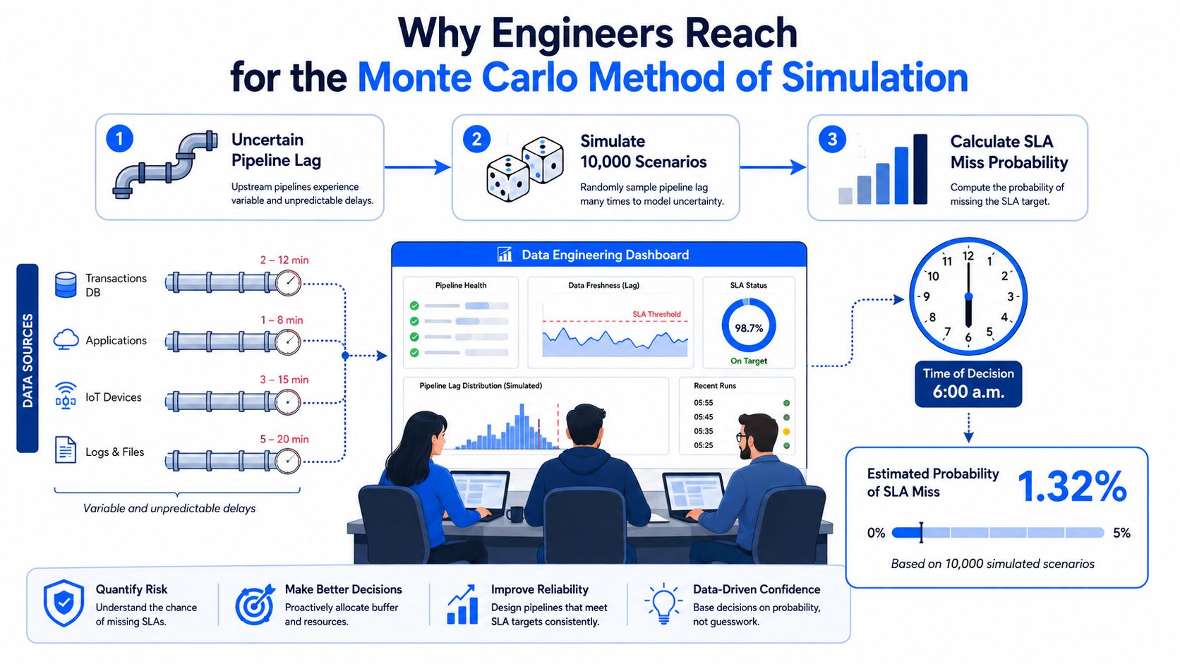
A data engineering team may know the historical behavior of each upstream source, yet still struggle to calculate the chance of missing a fixed delivery deadline analytically. One source can arrive late, another can fail and retry, and a third can deliver an unusually large batch that extends transformation time. Each branch changes the next one, so a single closed-form formula becomes difficult to maintain and harder to defend.

Monte Carlo simulation approaches the problem differently. The team represents uncertain inputs with realistic distributions, generates synthetic pipeline runs, evaluates whether each run finishes before the SLA, and aggregates the results into a probability estimate. The output isn't a promise that a particular run will be late. It's an evidence-based view of how the modeled system behaves across many plausible conditions.

From an impossible equation to a manageable experiment

The method's appeal isn't randomness for its own sake. It's the ability to replace an intractable analytic problem with a tractable computational experiment. Engineers can ask questions such as:

• Capacity planning: How much processing headroom does the workload need under high-volume arrivals?

• Risk review: How often do combinations of upstream delay and retry behavior create an SLA breach?

• Stakeholder commitments: How defensible is the proposed delivery time when inputs remain variable?

Each simulation run acts like a synthetic operational day. A run might draw a short upstream delay and modest row volume. Another might combine several late arrivals with additional retries. The model records the completion time and classifies the run as a success or breach.

Practical rule: Model the uncertainty that changes the decision. Adding random inputs that don't affect the SLA only increases complexity.

If you want a separate walkthrough of the basic workflow, the Polytreasury simulation tutorial provides useful introductory context. For enterprise data teams, the important shift is conceptual: stop asking for one supposedly precise completion time and start asking how the full range of plausible runs affects operational risk.

The Origins Behind the Monte Carlo Method of Simulation

The modern story begins with Stanisław Ulam, who was recovering from illness and thinking about solitaire. He wondered how likely a particular card layout was to produce a win. Counting every possible arrangement analytically would be impractical, but repeatedly dealing hands and recording the result was straightforward.

That insight changed the question. Instead of enumerating every outcome, Ulam could use random trials to estimate the percentage of wins. The same logic could apply to systems with enormous state spaces, where direct calculation becomes unrealistic.

Ulam shared the idea with John von Neumann at Los Alamos during the Manhattan Project. Von Neumann recognized its relevance to neutron diffusion and related nuclear-physics calculations. The method's modern computational form was intentionally developed in the mid-1940s, when the researchers needed a way to reason about complex physical behavior that resisted simpler analytical treatment.

Why the ENIAC milestone matters

A major milestone came in 1948, when von Neumann, Nicholas Metropolis, and others used the ENIAC computer to perform the first fully automated Monte Carlo calculations. The first unclassified paper followed in 1949. That transition matters because it moved the method from manual reasoning about chance into large-scale computer-based simulation.

Metropolis helped give the approach its memorable code name, drawing on the probabilistic character of the Monte Carlo casino in Monaco. The name stuck because it captures the central intuition: random trials can reveal the behavior of a complicated system.

The history has a direct lesson for data engineers. Monte Carlo wasn't born as an academic exercise detached from operations. It emerged because researchers faced a problem too complicated to solve conveniently with direct enumeration. Enterprise teams face the same pattern when hundreds of tables, schedules, retries, dependencies, and changing data volumes interact inside a production platform.

Core Principles That Make Random Sampling Work

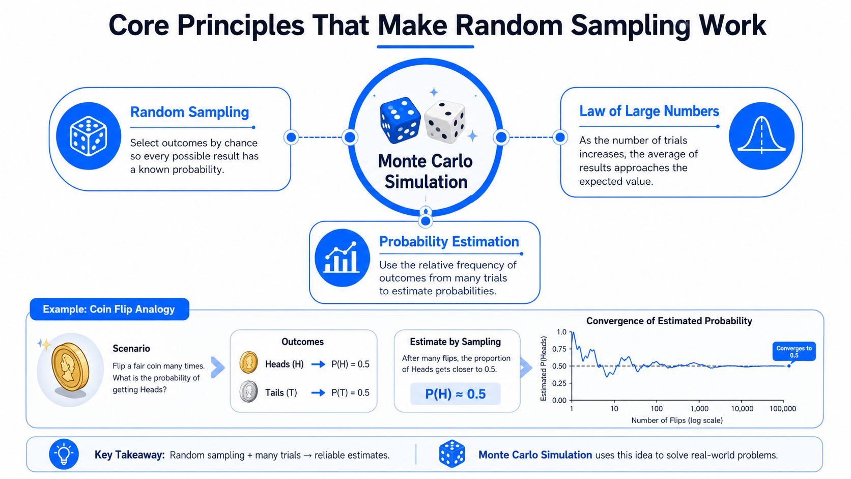
Suppose you want to estimate how often a fair coin lands heads. You could derive the probability mathematically, or you could flip the coin repeatedly and calculate the share of heads. The second approach is less elegant for a simple coin, but it gives you the right mental model for Monte Carlo simulation.

For an enterprise pipeline, the “coin” becomes a system model. Each trial samples uncertain inputs, runs those inputs through the model, and records an output such as completion time, failed validation count, or SLA status.

The four-stage algorithm

1. Define the input domain. Choose a probability distribution for each uncertain variable. Upstream lag might be modeled from historical arrivals, retry count from observed operational behavior, and row count from recent partitions.

2. Generate samples. A pseudorandom generator draws one value from each input distribution for every iteration. The generator is deterministic under a fixed seed, which makes a run reproducible.

3. Evaluate the system. Feed the sampled values into the pipeline model. The model might add task durations, apply retry rules, calculate resource consumption, or classify a run as an SLA breach.

4. Aggregate the outputs. Summarize the recorded results using a mean, percentile, or tail probability. For the SLA question, divide breach outcomes by total simulated runs to estimate the modeled breach probability.

Let the output from iteration (i) be (X_i). The expected value is approximated by the sample mean:

[

E[X] \approx \bar{X} = \frac{1}{N}\sum_{i=1}^{N}X_i

]

The sample variance can be written as:

[

Var(X) \approx s^2 = \frac{1}{N-1}\sum_{i=1}^{N}(X_i-\bar{X})^2

]

These formulas don't make the model correct by themselves. They summarize the behavior produced by the assumptions you supplied. A distribution that fails to represent seasonal arrivals, correlated upstream delays, or rare retry storms can produce a polished but misleading result.

For a broader grounding in statistical techniques used for data work, see statistical methods for data analysis. The central principle remains simple: repeated sampling produces an estimate, and the law of large numbers says that the estimate becomes more stable as the number of simulations grows.

Estimating Error and Convergence With Confidence

Monte Carlo output is an estimate, not an exact oracle. Two ideas explain why the estimate improves with more iterations. The law of large numbers describes convergence of the sample mean toward the true expected value, while the central limit theorem describes how the estimator tends to form a bell-shaped distribution around that value under suitable conditions.

For the sample mean, a common approximation for Monte Carlo standard error is:

[

SE = \frac{\sigma}{\sqrt{N}}

]

Here, (\sigma) represents the output standard deviation and (N) represents the iteration count. The square root matters operationally. Increasing the run count improves precision, but with diminishing returns. Doubling the iterations reduces the standard error by roughly the square root of two, not by half.

A practical conversion example

Assume a team is estimating a daily active user conversion rate with a model whose output variance is known from the modeled inputs. Each iteration samples plausible active-user volume and conversion behavior, then calculates the resulting rate. The team shouldn't choose an iteration count because it sounds large. It should choose a target interval width that matches the decision.

If leadership only needs a broad planning range, a moderate standard error may be acceptable. If the result controls a costly capacity or campaign decision, the team may require a narrower interval. The correct run count depends on output volatility, the desired precision, and the consequence of acting on an uncertain estimate.

The table expresses the scaling relationship rather than prescribing a universal run count. A rare-event estimate may need more care than an average conversion rate, particularly when only a small portion of iterations produce the event of interest.

Convergence diagnostics for production

A running-mean plot shows whether the estimated metric settles into a stable region. A trace plot can reveal patterns in the generated outputs, while the Monte Carlo standard error provides a quantitative stopping rule.

For practical guidance on describing output shape, use how to describe the distribution of data. In production, stop when the estimate meets the predefined precision target and additional runs no longer change the decision materially. That approach is more responsible than selecting a large iteration count and assuming the result must be reliable.

Variance Reduction Techniques Worth Knowing

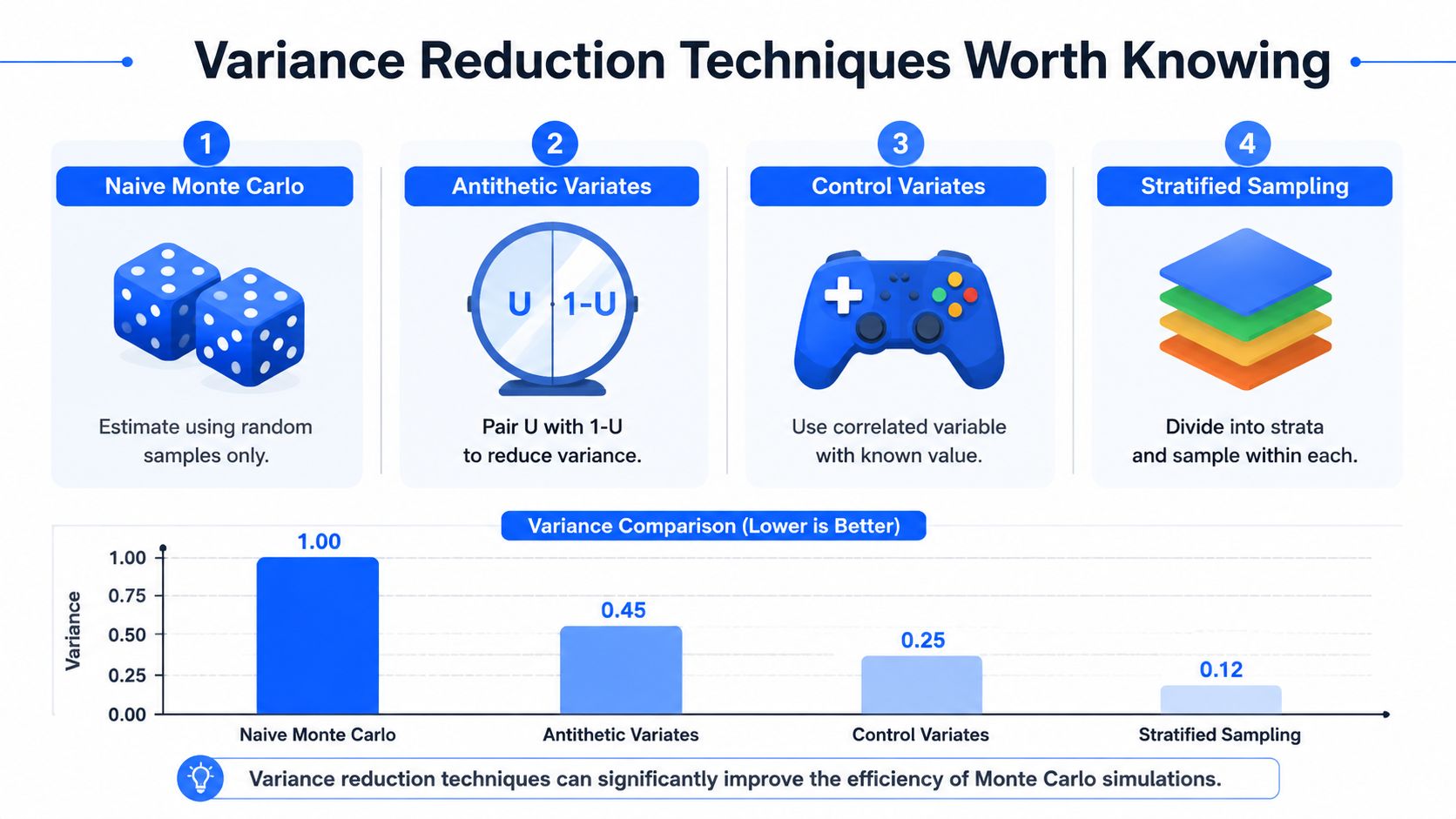
Naive Monte Carlo sampling is easy to explain and often a sensible baseline. It can also waste computation when the estimate is noisy, especially for rare events. Variance-reduction techniques improve precision by arranging or weighting samples more intelligently, without increasing the number of iterations.

Four approaches and their trade-offs

Antithetic variates pair a draw (U) with (1-U). If the model responds monotonically to the sampled input, the paired outputs can move in opposite directions and reduce variance. The cost is additional implementation logic and the requirement that the pairing makes sense for the model. This can suit a pipeline-duration model where one uniform input controls a monotone delay component.

Control variates use a correlated quantity whose expected value is known analytically. The simulation estimates the relationship between the target and the control, then subtracts the residual variation. This approach can be powerful, but it requires a useful control variable and careful coefficient estimation.

Stratified sampling divides the input domain into strata and samples within each region. It prevents the simulation from accidentally underrepresenting an important part of the range. For example, revenue percentile forecasts can reserve sampling coverage for low, typical, and high demand regions rather than relying on unrestricted random draws.

Importance sampling shifts the proposal distribution toward a rare-event region, then corrects the result with a likelihood ratio. It's a strong candidate for estimating SLA breach probabilities when breaches are uncommon, but incorrect weighting can introduce serious errors and obscure the interpretation of the output.

Modeling judgment: A variance-reduction method is useful only when its assumptions match the system. Lower numerical noise doesn't compensate for an incorrect dependency model.

Teams should document why they selected a technique, what bias correction it applies, and how they validated the result against a naive baseline. For unusual observations that feed the input model, outlier identification methods can help separate genuine extreme behavior from data errors before the simulation begins.

Pseudo-Code and In-Database Implementation Patterns

A reusable simulation template starts with the question, not the random generator. Define the output, identify uncertain inputs, select distributions, establish dependencies, and decide how the results will be consumed.

A compact version looks like this:

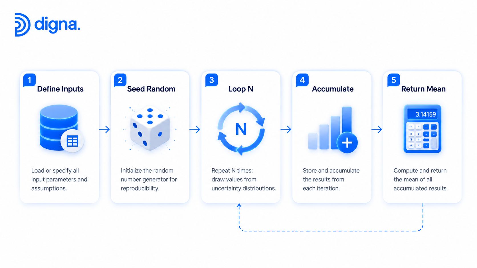
1. Define the input distributions and target output.

2. Initialize a pseudorandom source with a logged seed.

3. Draw one value from each distribution per iteration.

4. Evaluate the system model.

5. Store or accumulate the output.

6. Return summary statistics and selected percentiles.

7. Check convergence and validate the assumptions.

A Python reference model

The following example estimates the value at risk of a customer-churn loss distribution. It uses placeholders for the model parameters, so the point is the execution pattern rather than a claim about any particular business outcome.

import numpy as np

seed = 42
iterations = 10000
rng = np.random.default_rng(seed)

customer_count = rng.poisson(lam=1000, size=iterations)
churn_rate = rng.beta(a=2, b=98, size=iterations)
loss_per_customer = rng.lognormal(mean=3.0, sigma=0.6, size=iterations)

loss = customer_count * churn_rate * loss_per_customer

mean_loss = loss.mean()
standard_deviation = loss.std(ddof=1)
value_at_risk = np.quantile(loss, 0.95)

print(mean_loss, standard_deviation, value_at_risk)

import numpy as np

seed = 42
iterations = 10000
rng = np.random.default_rng(seed)

customer_count = rng.poisson(lam=1000, size=iterations)
churn_rate = rng.beta(a=2, b=98, size=iterations)
loss_per_customer = rng.lognormal(mean=3.0, sigma=0.6, size=iterations)

loss = customer_count * churn_rate * loss_per_customer

mean_loss = loss.mean()
standard_deviation = loss.std(ddof=1)
value_at_risk = np.quantile(loss, 0.95)

print(mean_loss, standard_deviation, value_at_risk)

import numpy as np

seed = 42
iterations = 10000
rng = np.random.default_rng(seed)

customer_count = rng.poisson(lam=1000, size=iterations)
churn_rate = rng.beta(a=2, b=98, size=iterations)
loss_per_customer = rng.lognormal(mean=3.0, sigma=0.6, size=iterations)

loss = customer_count * churn_rate * loss_per_customer

mean_loss = loss.mean()
standard_deviation = loss.std(ddof=1)
value_at_risk = np.quantile(loss, 0.95)

print(mean_loss, standard_deviation, value_at_risk)

A production implementation should record the seed, distribution parameters, model version, source partitions, and execution timestamp. It should also preserve enough metadata to reproduce the result after the underlying data changes.

Moving the computation beside the data

Python works well when the model is complex, the output is granular, or the team needs specialized scientific libraries. Enterprise data teams often need a different pattern. They want to sample historical warehouse data, join against production tables, and calculate quality metrics without exporting sensitive records.

Snowflake, BigQuery, and Databricks can support warehouse-native patterns using SQL random functions, common table expressions, array generators, or user-defined table functions. A typical design generates an iteration relation, samples input parameters for each iteration, joins those parameters to aggregated historical metrics, evaluates the target expression, and stores only the simulation outputs.

This pattern keeps source data in the warehouse, avoids unnecessary movement, and lets parallel workers handle iteration work through the platform's execution engine. The team can materialize compact result tables containing means, standard deviations, percentiles, and breach indicators instead of transporting raw columns.

For a practical discussion of keeping quality computation close to warehouse data, see in-database data quality execution.

Choose Python when the model needs specialized libraries or row-level simulation outputs. Choose SQL or a warehouse-native function when data residency, large source tables, governance, and aggregate result granularity matter most.

Applying the Monte Carlo Method of Simulation in Enterprise Data Quality

Data quality teams can use simulation to turn historical behavior into quantified operational risk. The useful unit isn't always a customer or transaction. It may be a table partition, a delivery event, a schema version, or a business metric observed over time.

Timeliness and pipeline freshness

A freshness model can sample from historical row-arrival behavior and calculate the probability that a dataset arrives after its expected delivery window. Instead of using one static threshold, the model can account for variation in source timing, batch size, upstream dependencies, and processing duration.

That output supports a more precise alerting decision. A team can distinguish an ordinary late arrival from a combination of conditions that creates meaningful downstream risk. It can also use the simulated completion distribution to support capacity planning and incident prioritization.

Schema drift and downstream impact

Schema simulations can represent possible structural changes, such as an added column, a removed field, or a data type modification. The model can then evaluate whether each change conflicts with downstream queries, dashboards, validation rules, or ingestion contracts.

The result is a probability-oriented view of change risk. A schema change may be harmless for one consumer but disruptive for another. Simulating the dependency graph helps teams focus review effort where a structural change is most likely to break a critical output.

Adaptive null-rate and anomaly monitoring

Null-rate distributions can be generated from bootstrap samples of recent partitions. Those samples preserve observed variation and can help thresholds adapt to seasonal behavior instead of relying on brittle static limits. The same approach can support anomaly detection for volumes, duplicate rates, freshness, and other quality metrics.

KPI volatility modeling adds another layer. A team can simulate revenue paths under correlated input noise, then present confidence bands that executives can interpret without mistaking a point forecast for certainty.

digna combines data anomaly detection, timeliness monitoring, validation, schema tracking, and business monitoring in an in-database platform. Its execution model keeps sensitive column data inside the customer's environment while producing statistical outputs that teams can use for observability decisions. The Monte Carlo approach to data observability shows how simulation can replace guesswork with quantified risk for the alerts a platform raises.

Common Misconceptions and a Practical Checklist

Monte Carlo simulation doesn't make a weak model trustworthy. Random draws can reproduce the wrong distribution with impressive consistency, and a large result set can make flawed assumptions look authoritative.

Four misconceptions cause recurring production problems:

• Random means correct: A pseudorandom generator samples from the distribution you specify. It can't determine whether that distribution reflects actual pipeline behavior.

• More iterations remove every error: More runs reduce sampling variance, but they don't remove bias caused by missing dependencies, poor data, or a misspecified model.

• A normal distribution fits by default: Operational data can be skewed, seasonal, bounded, or heavy-tailed. Distribution choice needs evidence from the source behavior.

• Variance reduction is automatically better: Antithetic, control, stratified, and importance sampling each introduce assumptions. A technique that fits one workload can distort another.

Quasi-random streams can sometimes reduce integration error for the same compute budget, but they require different reasoning from ordinary pseudorandom sampling. Treat them as a modeling choice to test, not a universal replacement.

A runbook checklist

Before a production simulation runs, verify the following:

• Validate distributions: Compare historical and fitted behavior with tests such as Kolmogorov-Smirnov or Anderson-Darling tests, then review the result with a domain owner.

• Set precision first: Define the desired confidence interval width before selecting the iteration count.

• Log the seed: Store the seed, input version, distribution parameters, and model version for reproducibility.

• Keep large data close: Prefer database-native sampling when source rows are large or sensitive.

• Review dependencies: Check whether upstream variables move together rather than assuming independence.

• Test rare events: Compare tail estimates with alternative sampling strategies and inspect their weighting.

• Revisit assumptions: Review distributions and variance-reduction choices on a regular operating cadence.

A responsible Monte Carlo workflow is statistical engineering, not a button labeled “run.” The model should make uncertainty visible, expose its assumptions, and give operators a clear reason to trust or challenge the output.

digna provides in-database data quality and observability capabilities for anomaly detection, timeliness, validation, schema tracking, and business monitoring. Use the Monte Carlo method of simulation to quantify pipeline and KPI risk where your data already lives, then visit digna to explore an enterprise deployment approach.