Monte Carlo Simulation: A Practical Guide for Data Teams

At 2 a.m., a monthly revenue dashboard jumps sharply. The on-call data engineer gets paged, checks the latest pipeline run, and finds no obvious error. The number could represent a real business shift, a partial upstream load, or a silent schema change that altered the metric. The response depends on instinct because the team has no quantified view of how likely each explanation is.

Monte Carlo simulation replaces that single guess with a distribution of plausible outcomes. By repeatedly sampling uncertain inputs, a team can estimate the likelihood that a pipeline will fail, a KPI will drift, or a timeliness SLA will be breached. The method has deep roots in probability and computing, but its practical value for data teams is straightforward: it turns uncertainty into an operational signal.

Table of Contents

• The Moment You Wish You Had Run a Monte Carlo

  • From intuition to probability

• What Monte Carlo Simulation Is

  • Why repeated sampling works

• How the Method Works Step by Step

• Sampling, Convergence, and Variance Reduction

  • Choosing the right sampling strategy

• Monte Carlo for Pipelines, KPIs, and Timeliness SLAs

  • Three observability stories

  • From distributions to alerts

• Scaling Monte Carlo Inside the Database

  • A practical scaling playbook

• Pitfalls, Validation, and Where Assumptions Break

  • Validation moves that catch bias

  • A post-change diagnostic checklist

• Turning Simulation Results into Operational Monitoring

  • An integration checklist

The Moment You Wish You Had Run a Monte Carlo

The engineer compares the revenue spike with yesterday's dashboard, checks row counts, scans recent deployment notes, and asks the upstream owner whether anything changed. Those checks are useful, but they answer only whether the team has found evidence of a problem. They don't answer the more important question: how likely is it that the reported revenue is wrong?

A deterministic check might say that the table arrived on time and contains the expected columns. A Monte Carlo model can go further by representing uncertainty in upstream delivery, null behavior, event arrival, and transformation outcomes. Each simulated run becomes a plausible version of the night's processing, and the resulting output shows how often the revenue metric lands inside or outside an acceptable range.

Practical rule: Treat a dashboard value as an observation with uncertainty, not as unquestionable truth.

That distinction changes the incident response. If most simulated outcomes support the observed jump and the pipeline inputs look normal, the engineer can investigate a genuine business event with greater confidence. If many plausible runs produce a materially different value under the same upstream conditions, the team has evidence to prioritize data validation before executives act on the dashboard.

From intuition to probability

The method isn't reserved for crisis analysis. A nightly simulation can estimate the probability that a multi-stage pipeline completes before its delivery target. A business-monitoring model can estimate whether a KPI movement is consistent with partial nulls and late-arriving records. A timeliness model can estimate how often a downstream slowdown pushes data beyond its service expectation.

The mental shift is small but important. Instead of asking, “Will this pipeline fail?” ask, “Across plausible versions of tonight, how often does it fail, and which assumptions drive that result?” That question gives data engineers a measurable basis for alerts, escalation, and prioritization.

Monte Carlo simulation was formalized during the Manhattan Project in the 1940s, when Stanislaw Ulam and John von Neumann applied repeated random trials to problems such as neutron diffusion that were impractical to solve directly. The name was adopted in 1949 by Nicolas Metropolis, connecting the method with chance and the Monaco casino, as described in this historical account of Monte Carlo methods.

What Monte Carlo Simulation Is

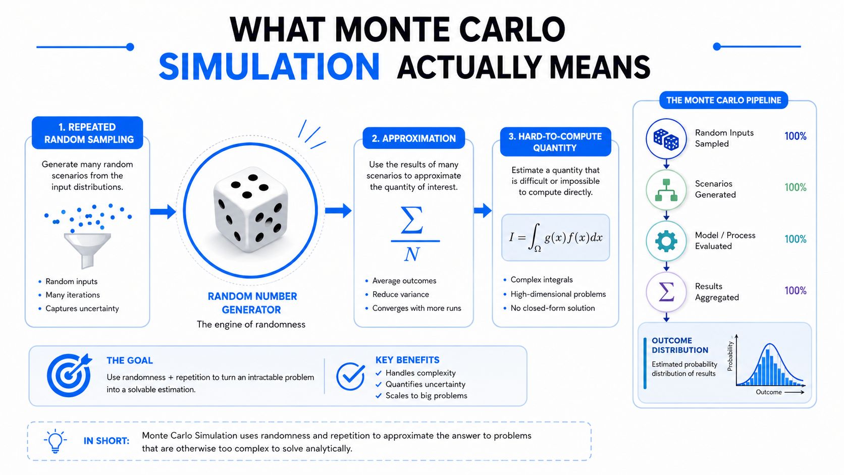
Monte Carlo simulation is repeated random sampling used to approximate a quantity that is difficult to compute analytically. The algorithm samples plausible states, evaluates the model for each one, and summarizes the results.

Consider a pipeline with five upstream stages. Each stage may fail, run late, or deliver incomplete data. Mental arithmetic can suggest the risk of one stage, but dependencies and changing conditions make the combined outcome difficult to calculate directly. The simulation represents each stage's uncertainty, creates one plausible version of a pipeline run, records whether it met its target, and repeats that process across many simulated runs.

Three building blocks define the mental model:

1. A system model: The stages, dependencies, transformations, and success criteria.

2. Uncertain inputs: Failure behavior, processing time, null rates, event delays, or other variables represented by probability distributions.

3. An output aggregator: A function that records each run's result, such as completion status, KPI value, or SLA breach.

The result is a distribution of answers, not one supposedly perfect value. Analysts can examine failure probability, the range of plausible KPI values, or the percentile of expected delivery time. This matters in observability because pipeline health rarely fits a clean binary boundary. A table may arrive on time while containing abnormal values, or pass validation while still increasing downstream risk.

Why repeated sampling works

Stanislaw Ulam's influential insight was to replace exhaustive calculation with many random trials. Britannica's account uses solitaire as an analogy: repeated games estimate the chance of winning without calculating every possible sequence. The same approach supports numerical integration, optimization, Bayesian statistics, and simulations of physical, biological, and social systems, as summarized in these Monte Carlo lecture notes.

For a data engineer, the casino metaphor is less useful than the separation between model structure and sampled inputs. Pipeline logic remains fixed while uncertain values change from run to run. The resulting distribution exposes risk hidden by a single-point forecast and gives an observability platform such as digna a way to connect simulated failure, KPI drift, and timeliness risk with operational monitoring.

How the Method Works Step by Step

Start by defining the pipeline outcome precisely. For example, a run is successful when every required stage completes before the delivery target and produces data that passes the relevant quality checks. A breach occurs when any required condition fails.

The algorithm then follows five practical steps:

1. Model the stages. List each upstream dependency and the way its state affects the final outcome.

2. Assign distributions. Represent uncertain failure behavior and processing time with distributions based on available history or domain judgment.

3. Draw one sample per stage. Each run creates one plausible version of the night.

4. Aggregate the result. Record whether the pipeline completed, breached its SLA, or produced an unacceptable KPI.

5. Repeat and inspect stability. Continue sampling until the key output estimates become sufficiently stable for the decision.

The following example uses NumPy for random sampling and pandas for summarization. It simulates one thousand pipeline nights, then calculates the observed share of runs that breached the SLA.

import numpy as np
import pandas as pd

# Create a reproducible random generator for repeatable development tests.
rng = np.random.default_rng(42)

# Define one thousand simulated pipeline nights.
n_runs = 1000

# Model five stages with illustrative, configurable failure probabilities.
failure_probabilities = np.array([0.02, 0.03, 0.01, 0.04, 0.02])

# Draw one failure state for every stage in every simulated night.
stage_failures = rng.random((n_runs, len(failure_probabilities))) < failure_probabilities

# A pipeline fails when at least one required stage fails.
pipeline_failed = stage_failures.any(axis=1)

# Store one row per simulation so the output can be audited or extended.
results = pd.DataFrame({
    "run_id": np.arange(n_runs),
    "pipeline_failed": pipeline_failed
})

# Estimate the probability of an SLA breach from the simulated outcomes.
sla_breach_probability = results["pipeline_failed"].mean()

print(f"Estimated SLA breach probability: {sla_breach_probability:.3f}")

import numpy as np
import pandas as pd

# Create a reproducible random generator for repeatable development tests.
rng = np.random.default_rng(42)

# Define one thousand simulated pipeline nights.
n_runs = 1000

# Model five stages with illustrative, configurable failure probabilities.
failure_probabilities = np.array([0.02, 0.03, 0.01, 0.04, 0.02])

# Draw one failure state for every stage in every simulated night.
stage_failures = rng.random((n_runs, len(failure_probabilities))) < failure_probabilities

# A pipeline fails when at least one required stage fails.
pipeline_failed = stage_failures.any(axis=1)

# Store one row per simulation so the output can be audited or extended.
results = pd.DataFrame({
    "run_id": np.arange(n_runs),
    "pipeline_failed": pipeline_failed
})

# Estimate the probability of an SLA breach from the simulated outcomes.
sla_breach_probability = results["pipeline_failed"].mean()

print(f"Estimated SLA breach probability: {sla_breach_probability:.3f}")

import numpy as np
import pandas as pd

# Create a reproducible random generator for repeatable development tests.
rng = np.random.default_rng(42)

# Define one thousand simulated pipeline nights.
n_runs = 1000

# Model five stages with illustrative, configurable failure probabilities.
failure_probabilities = np.array([0.02, 0.03, 0.01, 0.04, 0.02])

# Draw one failure state for every stage in every simulated night.
stage_failures = rng.random((n_runs, len(failure_probabilities))) < failure_probabilities

# A pipeline fails when at least one required stage fails.
pipeline_failed = stage_failures.any(axis=1)

# Store one row per simulation so the output can be audited or extended.
results = pd.DataFrame({
    "run_id": np.arange(n_runs),
    "pipeline_failed": pipeline_failed
})

# Estimate the probability of an SLA breach from the simulated outcomes.
sla_breach_probability = results["pipeline_failed"].mean()

print(f"Estimated SLA breach probability: {sla_breach_probability:.3f}")

The probabilities in this snippet are placeholders for model inputs, not production facts. A trustworthy implementation would estimate them from observed pipeline history, review dependencies between stages, and include processing-time behavior rather than treating every failure as identical.

For a complementary view of how statistical signals can support data monitoring, see statistical pattern recognition. The next challenge is making a working script dependable enough for operational decisions. That requires deliberate sampling, convergence checks, and variance reduction.

Sampling, Convergence, and Variance Reduction

Plain random sampling is the default because it's easy to implement and broadly applicable. Its error decreases with the square root of the number of samples, so additional runs improve precision gradually rather than magically eliminating uncertainty. This behavior follows from the law of large numbers, whose strong and weak forms underpin Monte Carlo convergence, as explained in this reference on Monte Carlo convergence.

That relationship matters when a team interprets a breach probability. A small change between two runs may reflect sampling noise rather than a meaningful change in the underlying pipeline. Track the running mean, inspect the Monte Carlo standard error, and compare estimates across independent workers or chains. A Gelman-Rubin R-hat check can help identify whether parallel chains have mixed, although it doesn't correct a badly specified model.

Choosing the right sampling strategy

Stratified sampling divides the input domain into disjoint strata and samples within each one. By removing the between-strata variance component, it can reduce variance substantially, especially when a pipeline has distinct operating regimes such as weekdays, month-end loads, or known release windows. The underlying mechanism is described in this technical reference on stratified sampling.

Importance sampling takes a different approach. It draws more samples from regions where the target function is larger, which can accelerate convergence when the event of interest is rare or highly concentrated, as described in this guide to improving Monte Carlo integration.

The broader variance-reduction family also includes common random numbers, conditioning, antithetic variates, control variates, stratified sampling, and importance sampling, as documented in this overview of Monte Carlo variance-reduction methods. For implementation guidance around statistical analysis in observability workflows, see statistical methods for data analysis.

Monte Carlo for Pipelines, KPIs, and Timeliness SLAs

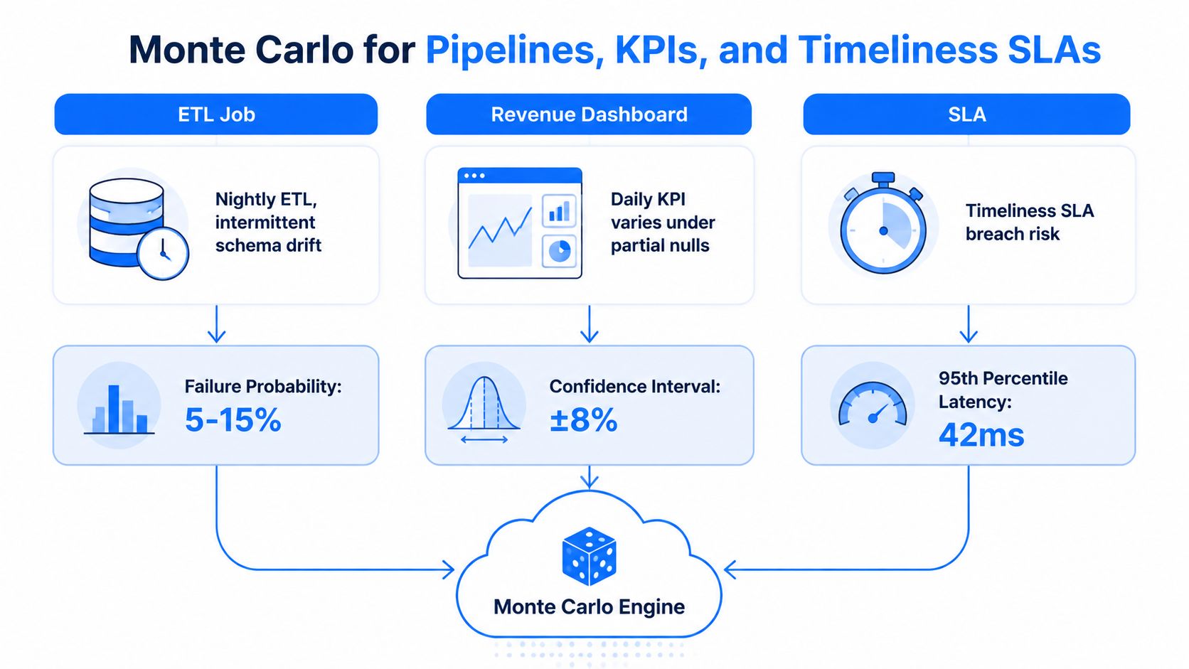
A nightly ETL may succeed most of the time while intermittent schema drift occasionally breaks a downstream transformation. A revenue dashboard may show a sharp movement because some records arrived late or a subset of values became null. A freshness SLA may remain technically compliant while processing latency steadily approaches its limit.

These are different operational problems, but they share the same shape. The inputs are uncertain, the model connects those inputs to an outcome, and the useful result is a probability distribution rather than a binary status.

Three observability stories

In the ETL case, the model samples stage availability, schema compatibility, and processing duration. Each run answers whether the complete workflow finishes before the expected delivery point. The monitoring output can become a failure-risk score, with lineage attached to the upstream tables and transformations that contribute most to the simulated risk.

For the revenue dashboard, the model samples partial null behavior, late-arriving events, and the effect of those conditions on the KPI calculation. Instead of declaring every movement anomalous, the team can compare the observed value with a simulated band and investigate when the observation falls outside the expected distribution.

Timeliness monitoring follows the same pattern. The model samples arrival and processing behavior, then evaluates whether the resulting delivery time crosses the SLA threshold. A breach probability can trigger an alert before the actual delivery misses its target, provided the inputs and dependencies are calibrated against operational history.

From distributions to alerts

An observability platform can use the simulation output in several ways:

• Failure risk: Alert when the probability of a pipeline failure crosses a team-defined threshold.

• KPI uncertainty: Show the observed metric beside its simulated range, then route investigation when the value departs from that range.

• SLA risk: Escalate when the predicted breach probability rises, even if the current load has not yet failed.

• Lineage context: Associate the result with the upstream datasets and transformations that influence the simulated outcome.

The alert shouldn't say only that a number is unusual. It should explain whether the unusual result is consistent with known input behavior, which assumptions drive the risk, and what downstream assets may be affected. Teams building timeliness checks can use this guide to data timeliness metrics to align simulation outputs with existing freshness definitions.

Scaling Monte Carlo Inside the Database

A notebook is a useful place to validate a model, but it becomes a poor execution boundary when the source data contains millions of rows and the simulation repeatedly needs the same warehouse-resident history. Pulling samples across the network adds data movement, creates another environment to secure, and separates the computation from the system that owns the operational data.

In-database execution reverses that boundary. SQL user-defined functions, array operations, and vectorized Python running on the data engine can keep sampling close to the source. The warehouse can allocate compute according to its execution model, while partition pruning limits reads to the relevant history.

A practical scaling playbook

Start with data locality. Store the historical inputs, distribution parameters, sampled values, and output summaries where downstream monitoring already runs. Avoid per-row random-function calls when a vectorized or warehouse-native random operation can generate batches more efficiently.

Then tune the execution plan:

• Batch by worker: Choose a batch size that keeps workers busy without exhausting memory.

• Prune partitions: Read only the time windows and assets needed for calibration.

• Vectorize calculations: Operate on arrays or sets rather than invoking the model row by row.

• Persist summaries: Store percentiles and breach probabilities instead of retaining every intermediate draw when audit requirements allow.

• Separate calibration from scoring: Refit distributions on a controlled schedule, then run lightweight scoring jobs more frequently.

A useful architecture test compares two workflows: running 100,000 iterations inside the database versus exporting samples to a notebook. The in-database option avoids network transfer and can reuse warehouse capacity, while the notebook option may require extra serialization, local memory, and data movement. The actual cost and latency depend on the engine, model complexity, partition layout, and worker allocation, so benchmark both paths with representative data rather than assuming one is universally cheaper.

For a broader explanation of keeping quality computation close to warehouse data, see in-database data quality execution. The design principle is simple: move the simulation logic to the data whenever repeated transfers would become the bottleneck.

Pitfalls, Validation, and Where Assumptions Break

More runs don't rescue a structurally unrealistic model. They can make a biased estimate appear stable because the simulation is repeatedly sampling from the same incorrect assumptions.

The most serious problems usually enter before execution:

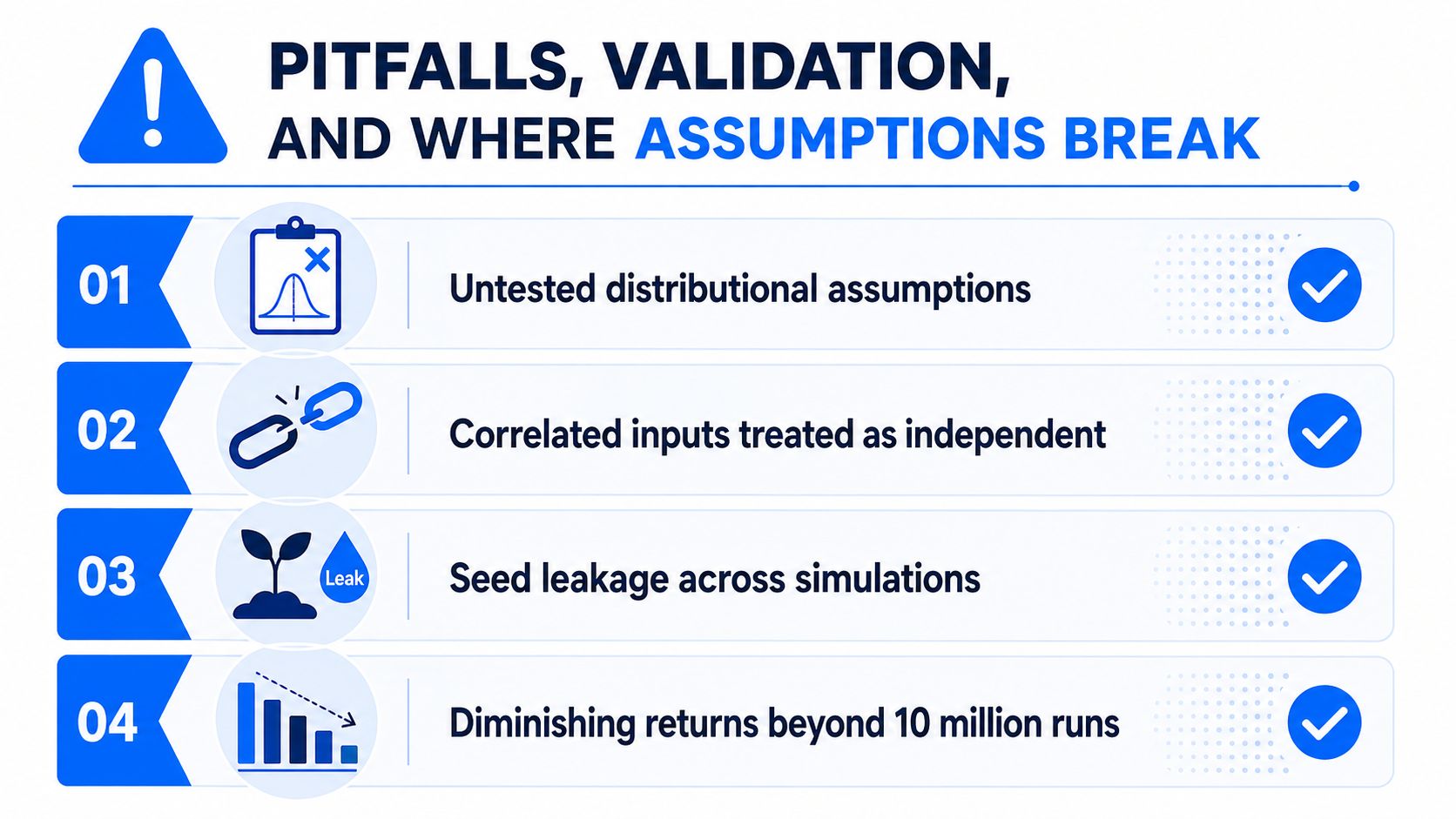
• Untested distributions: A normal or static distribution may not represent skew, regime changes, or operational tails.

• False independence: Correlated inputs, such as upstream delay and downstream queue time, may be sampled as if they were unrelated.

• Seed leakage: Shared or poorly managed random seeds can create unintended dependence across runs.

• Population drift: Silent schema changes or changing traffic composition can invalidate the historical population used for calibration.

• Narrow-regime convergence: A running estimate can look stable while excluding an important operating regime.

Recent risk-modeling literature highlights similar structural concerns, including static distributions, fixed correlation matrices, weak macroeconomic coherence, and high computational demand. The central lesson is that structural realism matters as much as random sampling, particularly in regulated finance and risk environments, as discussed in this analysis of Monte Carlo scenario-generation limitations.

Validation moves that catch bias

Backtest simulated failure rates against the last 90 days of incident logs, using the historical window as a validation reference rather than as proof that the future will behave identically. Check the fit of each marginal input distribution, inspect dependence between important variables, and run sensitivity sweeps on the 20% of parameters that drive 80% of the variance when those are established by your analysis, not assumed in advance.

Reproducibility also needs more than one fixed seed. Re-run the model with a fresh seed and compare the important percentiles, breach probabilities, and alert classifications. Large changes may indicate insufficient sampling, unstable tails, or an overly sensitive model.

A post-change diagnostic checklist

After each model change, verify:

1. The input population still matches the monitored assets.

2. Marginal distributions and dependencies remain plausible.

3. Independent seeds produce comparable decision outputs.

4. Convergence diagnostics cover the metrics used for alerting.

5. Backtesting doesn't reveal systematic underprediction of failures.

6. The model's assumptions and version are recorded with each result.

A simulation should earn operational trust through validation, not through the size of its iteration count.

Turning Simulation Results into Operational Monitoring

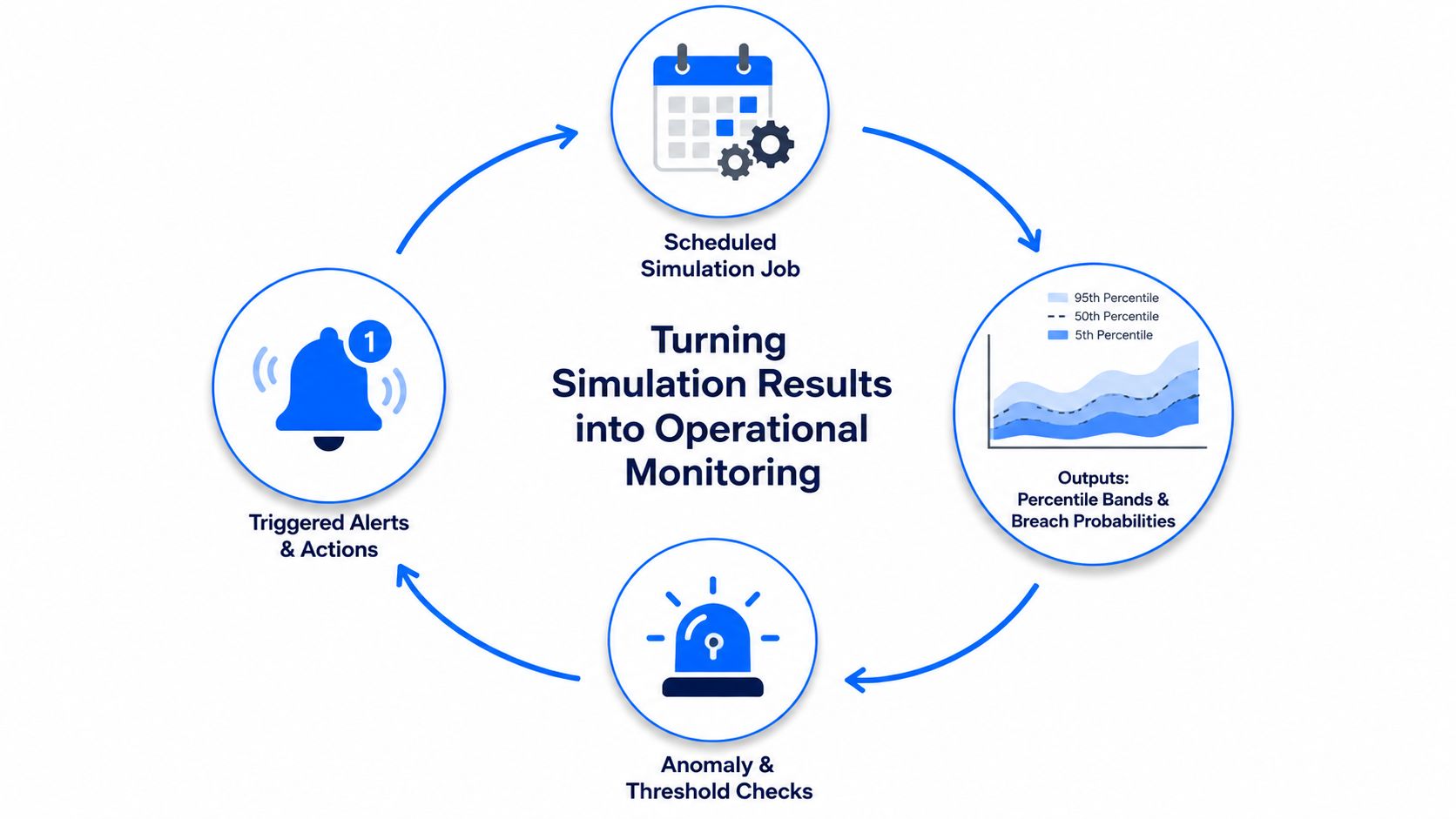
A production Monte Carlo workflow is a loop, not a notebook. A scheduled job calibrates or loads the current input distributions, runs the model, writes percentile bands and breach probabilities, and passes those outputs to the same anomaly and threshold checks that handle other observability signals.

The most useful daily table places predicted and observed values together. For a KPI, store the observed measurement, the relevant simulated range, the probability associated with the observed movement, the model version, and the timestamp of the run. For a pipeline, store the predicted failure risk, the actual result, and the upstream assets used to produce the estimate.

An integration checklist

• Schedule the model: Run calibration and scoring at frequencies appropriate to the behavior being monitored.

• Persist the evidence: Store distributions, seeds or seed policies, model versions, and output summaries.

• Connect the signal: Feed breach probabilities and percentile deviations into anomaly and threshold logic.

• Route the action: Send alerts to existing incident channels with lineage and suggested investigation context.

• Review outcomes: Compare predictions with observed failures and update assumptions when behavior changes.

This approach fits an in-database observability architecture, where simulations execute near the data and results land alongside validation, schema, anomaly, and timeliness metrics. A reporting layer such as data monitoring and reporting can then present the observed metric and its predicted distribution in the same operational view.

digna provides an enterprise platform that performs data-quality and observability analysis inside the customer's environment, including anomaly detection, timeliness monitoring, validation, schema tracking, and business or platform metrics. Visit digna to evaluate how its in-database approach could connect Monte Carlo risk signals with the monitoring workflows your data team already operates.