Monte Carlo Technique of Simulation: A Practical Guide

Your ETL job usually refreshes the customer table in about two hours. This morning, with a board meeting approaching, the same refresh is still running after six. Dashboards have turned red, downstream reports are stale, and the on-call engineer is checking cluster load, API logs, and warehouse queues at the same time.

The problem isn't that the team forgot how to estimate. The problem is that a single estimate hid the conditions that could make the job slow. Monte Carlo technique of simulation makes those conditions explicit, samples from their uncertainty, and turns one confident answer into a distribution of possible outcomes.

Table of Contents

• Why Deterministic Estimates Often Fail

  • A point estimate hides the spread

• The Core Idea Behind the Monte Carlo Technique of Simulation

  • Why repetition helps

  • The simulation loop

• Algorithms and Pseudocode You Can Reuse

  • Generic pseudocode

  • Patterns worth reusing

• Implementing Monte Carlo in Python, R, and SQL

  • Python with NumPy

  • R with replicate

  • SQL inside the warehouse

• Use Cases in Data Quality, Observability, and Risk

  • Row-count anomaly detection

  • Pipeline freshness risk

  • Financial and operational loss

• Pitfalls and Best Practices to Avoid

  • Randomness isn't automatically independent

  • Convergence needs evidence

• Putting Monte Carlo to Work in an Enterprise Data Platform

  • A practical operating design

Why Deterministic Estimates Often Fail

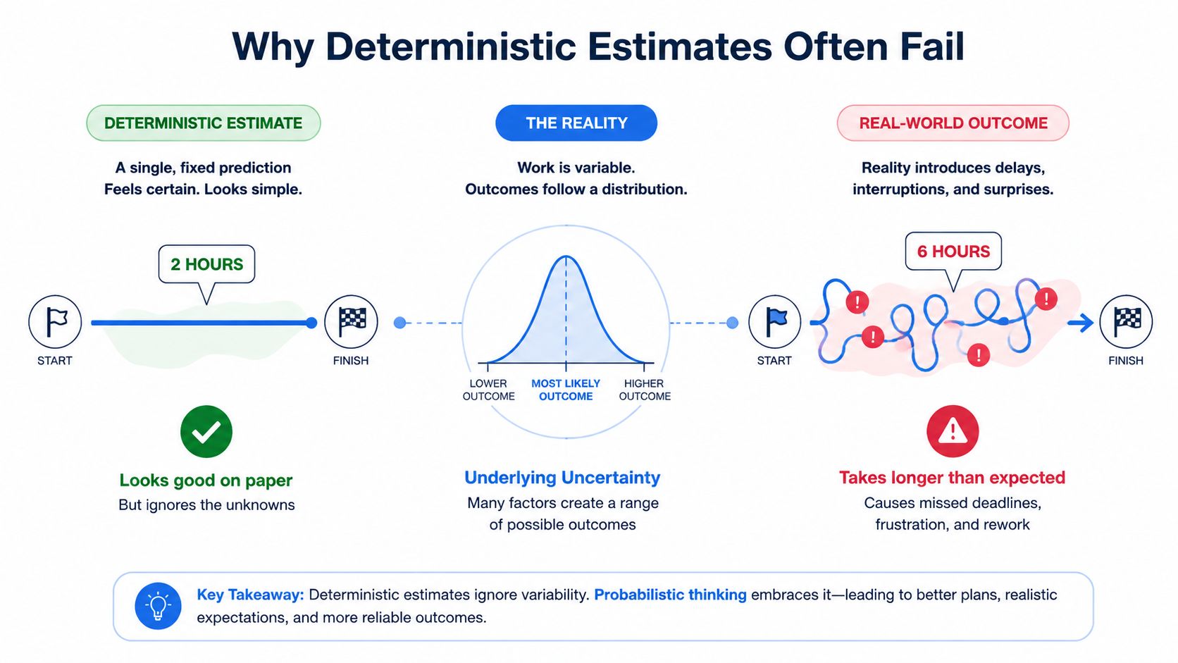
A deterministic estimate takes fixed inputs and produces a fixed output. For an ETL refresh, that might mean assuming a known payload size, predictable upstream latency, and a stable amount of compute capacity. The resulting promise sounds clear: the customer table will be ready within two hours.

That promise is useful only when the inputs are stable enough to justify it. In production, cluster contention can change during the run, an upstream API can respond slowly, and the incoming payload can be much larger than usual. A pipeline that normally completes quickly can encounter an unusual combination of conditions and miss its freshness expectation by a wide margin.

A point estimate hides the spread

Suppose an engineer records the duration of every successful refresh. The useful question isn't only, “What duration should we plan for?” It's also:

• Typical behavior: How long does the refresh usually take?

• Operational variation: How widely do durations spread?

• Tail behavior: How often does the job run unusually late?

• Decision threshold: At what probability should the team page someone?

A probability distribution describes that behavior more accurately than a single duration. It gives the team a way to distinguish ordinary variation from an event that deserves investigation. For a practical grounding in this idea, see what a distribution of data represents.

Randomness isn't automatically bad data. Some randomness reflects real operating conditions. The warehouse scheduler, network, source system, and workload all contribute variation that the pipeline must tolerate. Ignoring that variation doesn't remove it. It only moves the uncertainty into an incident.

Practical rule: If a decision depends on a range of plausible outcomes, model the range directly instead of hiding it behind an average.

A deterministic SLA can still be useful as a contract, but it shouldn't be mistaken for a complete forecast. The contract states what the business expects. A probabilistic model estimates how often the platform is likely to meet it under observed conditions.

The Monte Carlo technique of simulation treats the spread as an input, not an enemy.

The Core Idea Behind the Monte Carlo Technique of Simulation

The method becomes much easier once you hold three objects in your head. First, each uncertain input has a probability distribution. Second, the simulation takes a random draw from each distribution. Third, a model combines those draws and produces one output.

For a data pipeline, the inputs might include source extraction time, transformation time, warehouse queue delay, and final publication time. The model could add those durations, or it could include branching logic, retries, parallel tasks, and dependency rules. The model stays structurally the same while the sampled inputs change from one iteration to the next.

Why repetition helps

One random draw tells you almost nothing. It might land near the center of the distribution, or it might land in a tail. Repeating the process gives the output distribution enough observations to reveal its shape.

This is the intuition behind the law of large numbers. Individual samples remain noisy, but the aggregate behavior becomes more stable as the number of independent samples grows. In your mind, start with a rough histogram whose bars jump around. As more iterations arrive, the bars smooth out and the central pattern becomes easier to see.

The result isn't certainty. It's a more reliable approximation of the model implied by your inputs.

The simulation loop

Every iteration follows the same cycle:

1. Sample inputs: Draw a value from each input distribution.

2. Run the model: Feed those values into the aggregation or business logic.

3. Store the output: Keep the resulting duration, loss, row count, or other metric.

4. Repeat the process: Continue until the output is stable enough for the decision.

5. Summarize results: Inspect the mean, percentiles, and probability of crossing a threshold.

The output distribution answers questions a point estimate can't. You can ask how long a refresh usually takes, how late the slowest plausible paths become, or how likely a dashboard is to miss its freshness contract.

For a data-engineering view of this workflow, Monte Carlo methods for better data observability connects repeated sampling with operational monitoring.

The technique offers three practical promises: distributional answers, visibility into tail risk, and reproducible variability when the random generator is controlled. The algorithm below turns those promises into reusable implementation steps.

Algorithms and Pseudocode You Can Reuse

Start with the algorithm, not the programming language. The language is only the machinery used to execute the loop.

Generic pseudocode

define distribution for each uncertain input
create an empty output collection

repeat N times:
    draw one value from every input distribution
    pass the drawn values to the model
    store the model output

calculate summaries from the output collection
return the summaries and the output distribution

define distribution for each uncertain input
create an empty output collection

repeat N times:
    draw one value from every input distribution
    pass the drawn values to the model
    store the model output

calculate summaries from the output collection
return the summaries and the output distribution

define distribution for each uncertain input
create an empty output collection

repeat N times:
    draw one value from every input distribution
    pass the drawn values to the model
    store the model output

calculate summaries from the output collection
return the summaries and the output distribution

The important separation is between sampling and modeling. Sampling answers, “Which plausible input values should this iteration use?” The model answers, “What outcome follows from those values?” Mixing those responsibilities makes testing and debugging harder.

A practical Python example can estimate the probability that the sum of three lognormal job durations exceeds a four-hour SLA. The distribution is appropriate for a positive, right-skewed duration model, but the parameters below are illustrative placeholders for a demonstration, not production estimates.

import numpy as np

def estimate_sla_breach(
    iterations=100_000,
    seed=42,
    threshold_hours=4.0,
):
    # Create a reproducible random-number generator.
    rng = np.random.default_rng(seed)

    # Draw all durations in vectorized form.
    durations = rng.lognormal(
        mean=0.0,
        sigma=0.35,
        size=(iterations, 3),
    )

    # Add the three sampled job durations for every iteration.
    total_hours = durations.sum(axis=1)

    # Calculate the share of simulated outcomes above the SLA.
    breach_probability = np.mean(total_hours > threshold_hours)

    # Extract useful distribution summaries.
    summary = {
        "mean_hours": float(np.mean(total_hours)),
        "p50_hours": float(np.percentile(total_hours, 50)),
        "p95_hours": float(np.percentile(total_hours, 95)),
        "breach_probability": float(breach_probability),
    }

    return summary, total_hours

import numpy as np

def estimate_sla_breach(
    iterations=100_000,
    seed=42,
    threshold_hours=4.0,
):
    # Create a reproducible random-number generator.
    rng = np.random.default_rng(seed)

    # Draw all durations in vectorized form.
    durations = rng.lognormal(
        mean=0.0,
        sigma=0.35,
        size=(iterations, 3),
    )

    # Add the three sampled job durations for every iteration.
    total_hours = durations.sum(axis=1)

    # Calculate the share of simulated outcomes above the SLA.
    breach_probability = np.mean(total_hours > threshold_hours)

    # Extract useful distribution summaries.
    summary = {
        "mean_hours": float(np.mean(total_hours)),
        "p50_hours": float(np.percentile(total_hours, 50)),
        "p95_hours": float(np.percentile(total_hours, 95)),
        "breach_probability": float(breach_probability),
    }

    return summary, total_hours

import numpy as np

def estimate_sla_breach(
    iterations=100_000,
    seed=42,
    threshold_hours=4.0,
):
    # Create a reproducible random-number generator.
    rng = np.random.default_rng(seed)

    # Draw all durations in vectorized form.
    durations = rng.lognormal(
        mean=0.0,
        sigma=0.35,
        size=(iterations, 3),
    )

    # Add the three sampled job durations for every iteration.
    total_hours = durations.sum(axis=1)

    # Calculate the share of simulated outcomes above the SLA.
    breach_probability = np.mean(total_hours > threshold_hours)

    # Extract useful distribution summaries.
    summary = {
        "mean_hours": float(np.mean(total_hours)),
        "p50_hours": float(np.percentile(total_hours, 50)),
        "p95_hours": float(np.percentile(total_hours, 95)),
        "breach_probability": float(breach_probability),
    }

    return summary, total_hours

Patterns worth reusing

• Vectorized sampling: numpy.random.default_rng generates arrays efficiently instead of forcing Python to manage every draw in a slow loop.

• Controlled randomness: A seed makes a run reproducible, which matters when an engineer needs to explain an alert or compare model versions.

• Progress visibility: For a deliberately iterative or path-dependent model, wrap the loop with tqdm so a long-running job exposes its progress.

Readers moving from algorithm sketches into working Python can use these pseudo code to Python examples as a reference for translating logic cleanly.

You can later explore antithetic variates and control variates as variance-reduction techniques. They aren't required for a first model, but they can reduce simulation noise when each run is expensive. For anomaly workflows, the same output summaries can support data anomaly detection in Python.

Implementing Monte Carlo in Python, R, and SQL

The same simulation doesn't become mathematically different because it moves between Python, R, and SQL. The trade-off is operational: where should sampling happen, where should the model execute, and where will the results be consumed?

Python with NumPy

Python is usually the fastest place to prototype. NumPy handles vectorized sampling, percentile extraction is straightforward, and the surrounding ecosystem supports fitting distributions, plotting diagnostics, and testing model behavior.

import numpy as np

rng = np.random.default_rng(42)
samples = rng.lognormal(mean=0.0, sigma=0.35, size=(100_000, 3))
totals = samples.sum(axis=1)

result = {
    "p50": np.percentile(totals, 50),
    "p95": np.percentile(totals, 95),
    "probability_above_sla": np.mean(totals > 4.0),
}

import numpy as np

rng = np.random.default_rng(42)
samples = rng.lognormal(mean=0.0, sigma=0.35, size=(100_000, 3))
totals = samples.sum(axis=1)

result = {
    "p50": np.percentile(totals, 50),
    "p95": np.percentile(totals, 95),
    "probability_above_sla": np.mean(totals > 4.0),
}

import numpy as np

rng = np.random.default_rng(42)
samples = rng.lognormal(mean=0.0, sigma=0.35, size=(100_000, 3))
totals = samples.sum(axis=1)

result = {
    "p50": np.percentile(totals, 50),
    "p95": np.percentile(totals, 95),
    "probability_above_sla": np.mean(totals > 4.0),
}

R with replicate

R is a strong choice when the work centers on statistical analysis and visualization. replicate() makes repeated evaluation readable, while packages such as dplyr can shape summaries after the simulation.

set.seed(42)

one_run <- function() {
  durations <- rlnorm(3, meanlog = 0, sdlog = 0.35)
  sum(durations)
}

totals <- replicate(100000, one_run())

summary <- data.frame(
  p50 = quantile(totals, 0.50),
  p95 = quantile(totals, 0.95),
  probability_above_sla = mean(totals > 4.0)
)

set.seed(42)

one_run <- function() {
  durations <- rlnorm(3, meanlog = 0, sdlog = 0.35)
  sum(durations)
}

totals <- replicate(100000, one_run())

summary <- data.frame(
  p50 = quantile(totals, 0.50),
  p95 = quantile(totals, 0.95),
  probability_above_sla = mean(totals > 4.0)
)

set.seed(42)

one_run <- function() {
  durations <- rlnorm(3, meanlog = 0, sdlog = 0.35)
  sum(durations)
}

totals <- replicate(100000, one_run())

summary <- data.frame(
  p50 = quantile(totals, 0.50),
  p95 = quantile(totals, 0.95),
  probability_above_sla = mean(totals > 4.0)
)

SQL inside the warehouse

SQL wins when the simulation depends on data already stored in the warehouse. Pulling large historical samples into Python adds network movement, memory pressure, and another execution boundary. A warehouse implementation can join historical duration records to a random reference table, calculate simulated outcomes beside the source data, and persist summaries without exporting raw rows.

The exact random function differs by database, so isolate it behind a small adapter. A recursive CTE can generate iteration identifiers, while a join to sampled reference rows supplies input values. For high-volume daily row-count checks, this keeps computation close to the partitions being tested.

A Python service can also use the digna Python SDK when the surrounding workflow needs to connect simulation outputs with platform monitoring. The decision should follow data locality and model complexity, not team preference alone.

Use Cases in Data Quality, Observability, and Risk

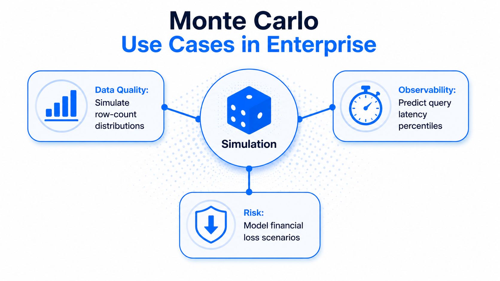
Monte Carlo becomes valuable in a data platform when a static threshold is too blunt. A row count can be valid in one operating period and suspicious in another. A pipeline can be late because of an unusual but legitimate workload. A fraud-loss distribution can look harmless at its center while carrying meaningful exposure in its tail.

Row-count anomaly detection

Start with historical hourly or daily partition counts. Instead of setting one fixed minimum and maximum, fit a distribution that reflects normal volume for the relevant period, day type, or source behavior. Simulate expected counts and compare the observed partition with the resulting range.

The action should depend on the decision boundary. A count outside the expected envelope can trigger investigation, while a count deep in the simulated tail can create a higher-priority incident. This approach can catch unusual spikes and drops that a broad static range would ignore.

Pipeline freshness risk

For timeliness, the input distribution is historical stage duration or arrival lag. The model combines those sampled delays with the scheduled dependency chain and estimates whether the downstream dashboard will be ready before its freshness contract.

This produces an operational probability rather than a vague warning. If the simulated late-arrival risk crosses the team's configured threshold, the platform can alert the owner before a stakeholder notices stale data. Engineers can then inspect the slowest stage instead of waiting for the final dashboard to fail.

Financial and operational loss

The same mechanics apply to revenue shortfall, fraud loss, or portfolio exposure. The input distribution may come from historical loss observations, fitted financial returns, or a deliberately stressed scenario. The output is a loss distribution, from which a risk team can inspect a percentile or estimate the chance of exceeding a defined tolerance.

A percentile isn't a guarantee. It's a statement about the assumptions and sampling process used to produce it.

Schema drift fits the same pattern. Sample null rates or type-change behavior across comparable datasets, then flag a newly observed rate that sits unusually far into the simulated distribution. That can expose silent breakage even when the pipeline technically completes.

Pitfalls and Best Practices to Avoid

Monte Carlo code can run successfully while producing a misleading answer. Production failures usually come from assumptions, dependencies, or diagnostics rather than from the loop itself.

Randomness isn't automatically independent

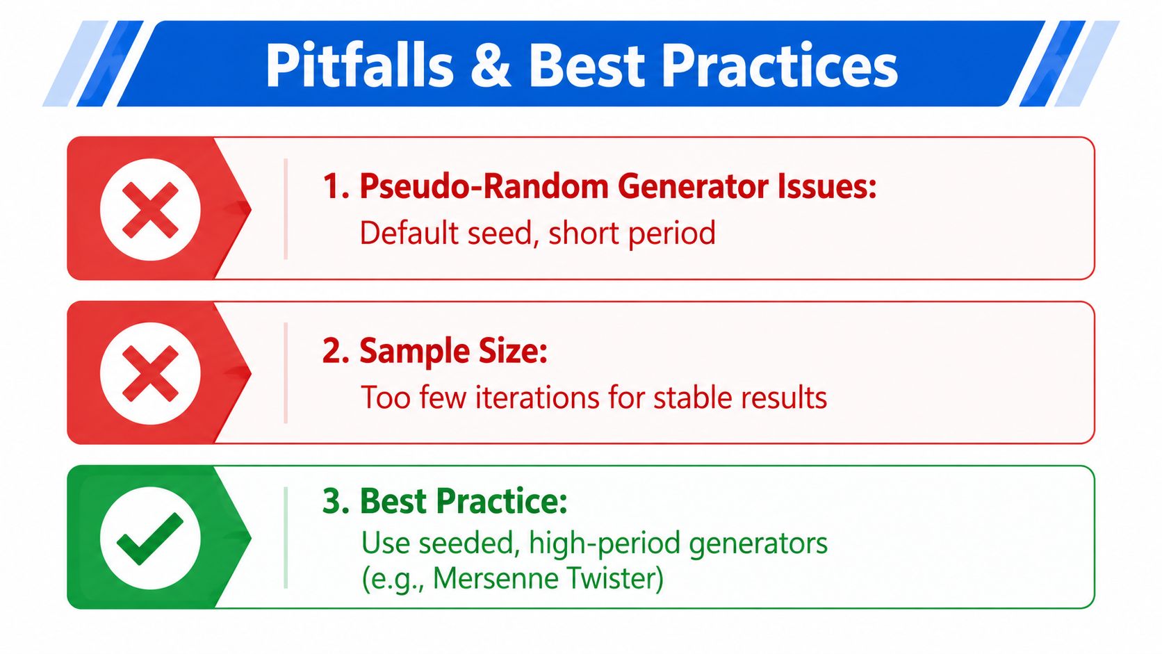
A pseudo-random generator is deterministic machinery designed to behave like random sampling. Poor defaults, short periods, or database-specific rand() behavior can create patterns that contaminate results. Seed the generator deliberately, use a well-understood implementation, and test the sampled distribution instead of assuming the function is suitable.

Correlated inputs are a more serious modeling error. If upstream latency and warehouse queue time rise together during load, sampling them independently will make the tail look calmer than reality. Use joint historical samples, a dependency model, or a copula when the relationship matters.

Convergence needs evidence

A running mean that appears flat doesn't prove that the tails have stabilized. Track the statistics that drive the decision, inspect trace plots, and compare results across independent batches. For models that use formal iterative sampling, Gelman-Rubin diagnostics can help assess whether chains have mixed adequately, although they don't repair a misspecified model.

Tail quantiles need special care. If your alert depends on a rare boundary, an apparently smooth center can coexist with an unstable tail. Increase the simulation effort, use variance-reduction methods where appropriate, and report uncertainty around the estimated percentile.

1. Fit distributions carefully: Use relevant history, segment unlike operating conditions, and document expert assumptions.

2. Control reproducibility: Store the seed, generator details, model version, and input parameters for every run.

3. Validate independently: Compare simple models with analytic results or known test cases before trusting production outputs.

4. Test dependencies: Measure relationships between inputs and preserve them when sampling.

5. Record audit metadata: Keep iteration settings, distribution choices, code versions, and summary results together.

Never treat the mean as ground truth. A Monte Carlo result is conditional on the model, the data, and the sampling process. More iterations can make a wrong model look more precise, not more correct.

Putting Monte Carlo to Work in an Enterprise Data Platform

Operational Monte Carlo belongs in the platform's normal execution path, not in an abandoned notebook. Schedule simulations alongside ETL, version their parameters, and write the resulting summaries back as monitored metrics. A model that can't be rerun and explained isn't ready for an enterprise alert.

A practical operating design

Keep the service boundary thin. Ingestion should provide the historical observations, the simulation component should sample and calculate, and the alerting layer should evaluate thresholds and notify owners. That separation lets engineers change the model without rewriting every downstream consumer.

Prefer in-database execution for high-volume checks such as partition counts, null-rate distributions, and freshness envelopes. Use Python or R for path-dependent models, bootstrap workflows, or simulations that require specialized statistical libraries. The right boundary is usually determined by data movement and model complexity.

Store enough metadata to reproduce every decision:

• Input distribution: Record the fitting method, parameters, source window, and segmentation logic.

• Simulation configuration: Persist the sample count, random generator, seed, and model version.

• Output summaries: Save percentiles, tail probabilities, means, and convergence diagnostics.

• Alert context: Attach the threshold, observed value, affected dataset, and owner response.

• Execution evidence: Keep run status, timestamps, and environment details for audit review.

A platform such as digna's enterprise data platform can provide the surrounding monitoring context for data behavior, timeliness, validation, and schema changes. The simulation output should appear beside ordinary freshness and quality signals, so teams can compare predicted risk with observed incidents.

Before release, verify that the model handles missing history, late-arriving records, changing schemas, retries, and partial warehouse failures. Then run it in shadow mode, compare alerts with engineer judgment, and tune thresholds only after reviewing false positives and missed events.

digna combines data anomaly detection, timeliness monitoring, validation, and schema tracking so teams can turn probabilistic signals into operational action. Visit digna to see how Monte Carlo-informed observability can fit inside your own enterprise data environment.