How to Use the Simulation and Monte Carlo Method

A pipeline cost forecast can look precise right up until the upstream system slows down, retries multiply, or a source begins sending incomplete records. Leadership may ask for one number for next quarter, while the data team knows only that latency, retry behavior, and null rates fall within broad, uncertain ranges. Averages make the forecast easy to present, but they can hide the outcomes that create the largest operational risk.

Simulation gives you a way to replay those uncertain conditions before they affect production. Instead of asking only, “What will the pipeline cost under typical conditions?”, you can ask, “How does the cost change across many plausible combinations of latency, retries, and missing data?” The result is a distribution that exposes risk, tests alert thresholds, and turns assumptions into something your team can inspect.

The Monte Carlo method is the most widely used engine for this translation. It repeatedly samples uncertain inputs, runs a model, and aggregates the outputs. The method originated at Los Alamos in the mid-1940s and moved quickly from wartime physics into a broad computational technique, as documented by the Los Alamos account of the method's birth. This guide connects its foundations to data observability, with practical Python and R patterns for metric ranges, pipeline stress tests, missing-data sensitivity, and anomaly-detection validation.

Table of Contents

• Why Data Teams Need Simulation

  • From point estimates to risk distributions

  • A production-oriented mindset

• Understanding Simulation and the Monte Carlo Method

  • The dartboard analogy

  • Mapping the loop to observability

• Key Statistical Foundations

  • Planning trials from a target interval

  • Reducing variance carefully

• Implementing the Monte Carlo Method

  • A compact implementation pattern

  • Python with NumPy

  • R with base functions

  • Engineering choices that matter

• Practical Applications for Data Teams

  • Metric ranges instead of false precision

  • Stress and sensitivity

  • Testing anomaly detectors

• Common Pitfalls and Best Practices

  • Reproducibility and input quality

  • Dependence and convergence

  • Avoiding validation overconfidence

• Building Reliable Simulation Studies

Why Data Teams Need Simulation

A data platform team is preparing a forecast for next quarter's pipeline cost. The finance model needs expected workload, but the inputs aren't fixed. An upstream API can arrive early or late, retry behavior changes under load, and source tables can contain more nulls than the team expects. A single average for each variable produces a clean spreadsheet, yet it says little about the combinations that push the platform beyond its budget or service objective.

A simulation changes the question. The team can generate many synthetic replays, sampling plausible arrival delays, retry rates, and null percentages for each trial. Every replay produces an outcome, such as processing time, compute consumption, failed records, or estimated cost. The collection of outcomes shows whether the decision is stable or whether a small change in assumptions creates a meaningful tail of bad results.

From point estimates to risk distributions

A deterministic calculation uses fixed inputs and returns one result. That approach is useful when the inputs are known and stable, but observability decisions rarely fit that description. A freshness threshold may depend on variable arrival behavior. A volume alert may depend on seasonality, delayed loads, and upstream filtering. A quality check may react differently depending on whether missing values are random or concentrated in a high-value segment.

Simulation lets engineers vary those inputs together. You can then inspect a median, a high-end outcome, a failure probability, or the range in which most trials fall. The point isn't to make uncertainty disappear. It's to make the uncertainty visible before a dashboard, alert, or capacity plan encodes an unjustified assumption.

Practical rule: If a decision depends on inputs you can describe only as ranges or distributions, a single estimate probably hides information your stakeholders need.

A production-oriented mindset

A useful simulation study starts with a decision, not a random-number generator. Define the outcome that matters, identify the uncertain inputs, document how those inputs relate, and preserve the trial results for review. The same harness can support a cost forecast, a pipeline stress test, or a check of whether an anomaly threshold remains useful when traffic changes.

The sections that follow turn that mindset into a working pattern. You'll see how the general idea of simulation differs from the Monte Carlo method, how convergence affects trust, how to implement the loop in Python and R, and how to connect the output to observability workflows.

Understanding Simulation and the Monte Carlo Method

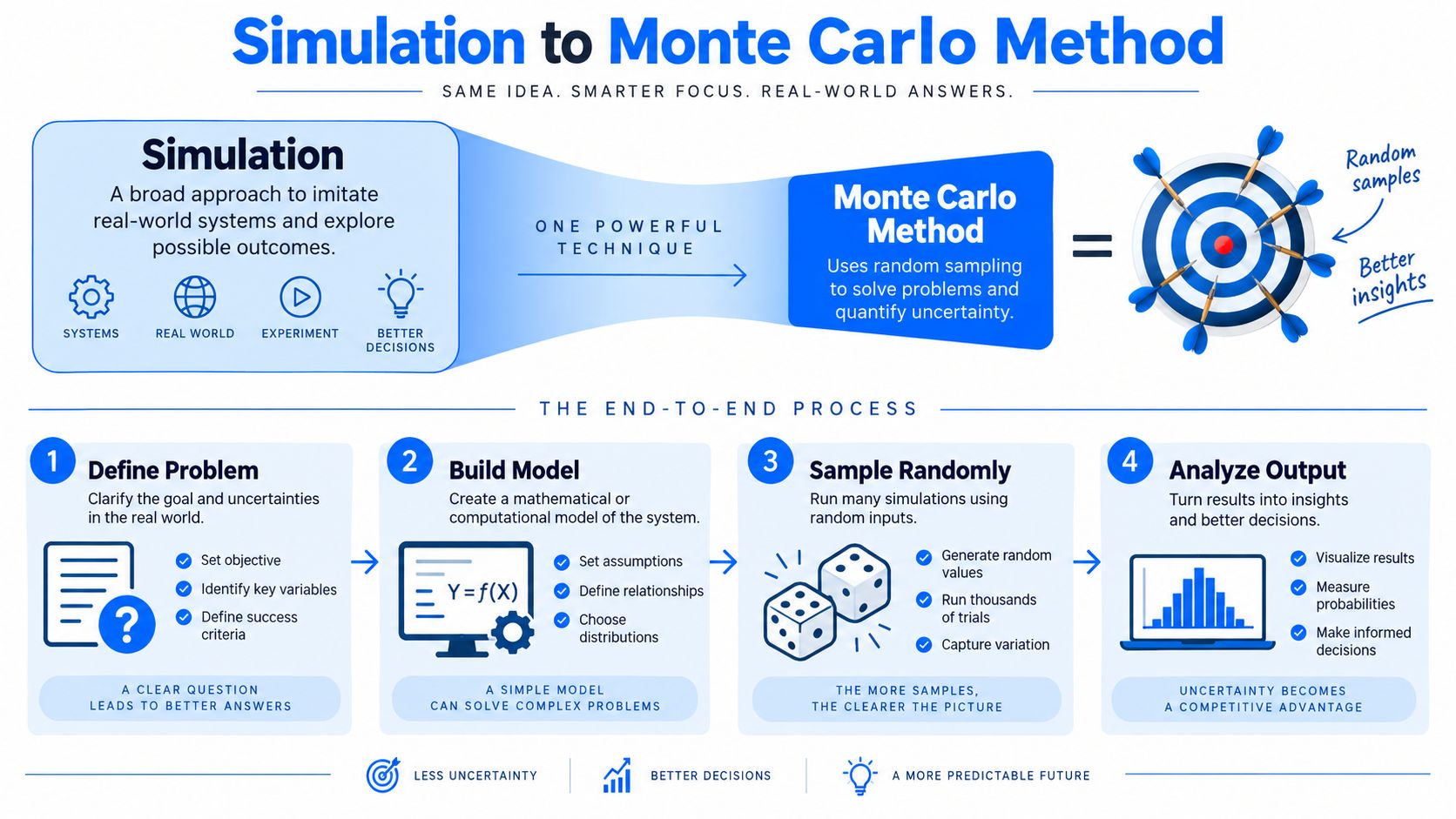
Simulation is the broad practice of imitating a real process with a model. A data engineer might simulate a pipeline by generating arrivals, applying transformations, injecting failures, and measuring completion time. The model may represent events over time, dependencies between services, or the effect of operational rules.

The Monte Carlo method is a family of techniques that uses repeated random sampling to estimate a numerical result or output distribution. A simulation can be deterministic, event-driven, or rule-based. Monte Carlo adds randomness to the inputs, the process, or both, then uses repeated trials to approximate what direct calculation may be unable to solve conveniently.

The dartboard analogy

Consider a square containing a circular dartboard. Throw random points across the square and record whether each point lands inside the circle. The fraction of points inside the circle estimates the circle's area relative to the square, which can then estimate pi when the geometry is defined appropriately.

The example is useful because it exposes the core loop:

1. Define the domain. Establish the square and the circle.

2. Sample inputs. Generate random coordinates.

3. Evaluate the model. Check whether each point falls within the circle.

4. Aggregate outputs. Convert the count of hits into an estimate.

The darts don't discover a hidden formula. They approximate an answer through repeated observations. More trials generally make the estimate less sensitive to the particular random sequence, although the quality of the result still depends on the model and sampling design.

Mapping the loop to observability

In a data platform, the square becomes the space of plausible operating conditions. Random coordinates become sampled arrival rates, processing times, failure events, or missingness patterns. The circle test becomes the pipeline, validation rule, or anomaly detector you want to evaluate. The aggregated result might be a latency quantile, a missed-alert rate, or the range of a business metric.

A trial is one execution of the model with one sampled set of inputs. A replication is a repeated execution intended to produce another comparable observation, often under the same model and sampling assumptions. An estimator is the calculation applied to trial outputs, such as a mean, quantile, or fraction exceeding a threshold.

The sampling distribution describes how that estimator varies across repeated samples. Convergence means the estimator becomes sufficiently stable for the decision you're making. It doesn't mean the model is correct. A converged simulation with poor input assumptions can produce a precise answer to the wrong question.

For a practical observability framing, see digna's guide to Monte Carlo methods for better data observability. The important engineering habit is to keep the stochastic inputs separate from deterministic business logic. That separation makes it possible to replace one input assumption, rerun the same model, and see which conclusions change.

Key Statistical Foundations

Monte Carlo results are estimates, not guarantees. If each trial produces an output (Y_i), a simple estimator for the expected output is the sample mean:

[
\hat{\mu} = \frac{1}{N}\sum_{i=1}^{N}Y_i
]

Under suitable independence and finite-variance assumptions, the standard error of that estimate is approximately:

[
SE(\hat{\mu}) = \frac{s}{\sqrt{N}}
]

Here, (s) is the observed sample standard deviation and (N) is the number of trials. The relationship matters operationally. The error shrinks at a rate proportional to one over the square root of N, so quadrupling the sample size halves the standard error. More trials help, but they don't usually produce linear gains.

Planning trials from a target interval

Start with a pilot run and measure the output variance. If you want a two-sided confidence interval with approximate half-width (h), and you use a normal critical value (z), a practical planning formula is:

[
N \approx \left(\frac{z s}{h}\right)^2
]

The formula is an approximation, not a substitute for checking convergence. It's most useful when the estimator is a mean and the output behaves reasonably. Quantiles, rare-event probabilities, heavy-tailed outputs, and dependent samples need more careful diagnostics because their uncertainty may be much larger than a mean-based calculation suggests.

Track the estimate cumulatively rather than inspecting only the final value. Plot the running mean or target quantile against the number of trials, and compare independent batches. If the result moves substantially when another batch arrives, the simulation isn't ready for a firm operational conclusion.

A separate concern is effective sample size. If trials are correlated, the nominal value of (N) overstates the amount of independent information. This commonly appears when engineers reuse a time-series trace, carry state between trials, or sample related inputs independently even though production shows them moving together.

Reducing variance carefully

Variance-reduction methods can improve precision without just running more trials. They can also make the model harder to explain, so use them when the baseline simulation is correct and the remaining uncertainty is worth optimizing.

For broader context on choosing statistical techniques, use digna's reference on statistical methods for data analysis. In a design review, explain not just that variance fell, but which assumption makes the technique valid and how you verified the weighting or pairing logic.

Implementing the Monte Carlo Method

A repeatable implementation separates the model from the random inputs. That design lets you test alternative distributions without rewriting pipeline logic.

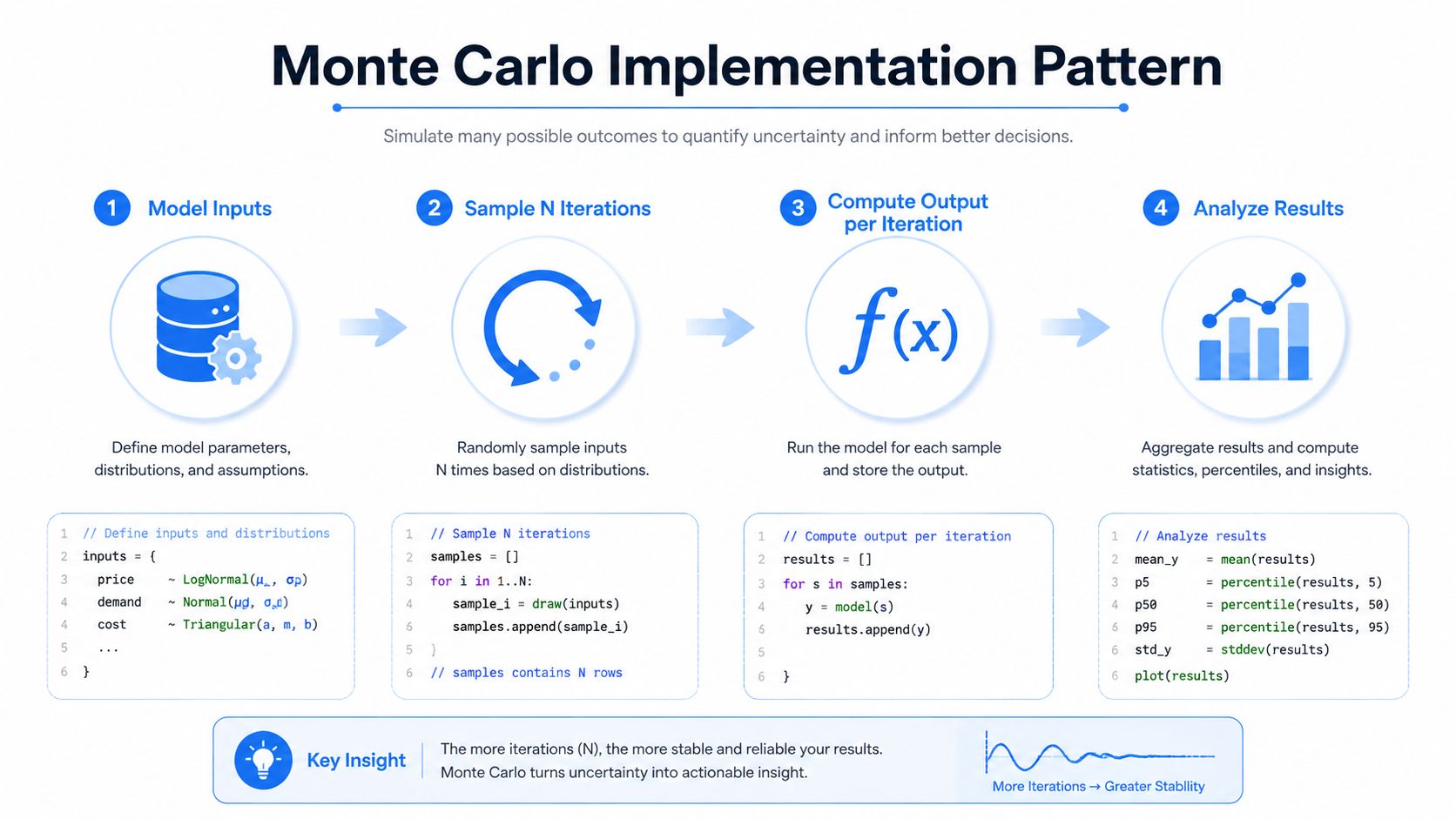
A compact implementation pattern

Use this pseudo-code as the skeleton:

1. Define model inputs and their distributions.

2. Set a seed strategy and choose (N) iterations.

3. Sample the uncertain inputs.

4. Compute one output for each iteration.

5. Aggregate the trial outputs.

6. Report the estimate and an uncertainty interval.

7. Save raw outputs and diagnostic information.

The model should be deterministic once its sampled inputs are supplied. If the output calculation includes hidden randomness, expose it as another input stream so you can reproduce and audit it.

Python with NumPy

The following example estimates a pipeline latency quantile when service time is right-skewed. A lognormal distribution is a reasonable demonstration for positive, skewed service times, but production parameters should come from observed data or a documented assumption.

import numpy as np

rng = np.random.default_rng(42)

iterations = 100_000
requests_per_run = 500

service_time = rng.lognormal(
    mean=np.log(0.08),
    sigma=0.55,
    size=(iterations, requests_per_run),
)

run_latency = service_time.sum(axis=1)
p95_latency = np.quantile(run_latency, 0.95)

lower = np.quantile(run_latency, 0.025)
upper = np.quantile(run_latency, 0.975)

print({
    "p95_latency": p95_latency,
    "interval_lower": lower,
    "interval_upper": upper,
})

import numpy as np

rng = np.random.default_rng(42)

iterations = 100_000
requests_per_run = 500

service_time = rng.lognormal(
    mean=np.log(0.08),
    sigma=0.55,
    size=(iterations, requests_per_run),
)

run_latency = service_time.sum(axis=1)
p95_latency = np.quantile(run_latency, 0.95)

lower = np.quantile(run_latency, 0.025)
upper = np.quantile(run_latency, 0.975)

print({
    "p95_latency": p95_latency,
    "interval_lower": lower,
    "interval_upper": upper,
})

import numpy as np

rng = np.random.default_rng(42)

iterations = 100_000
requests_per_run = 500

service_time = rng.lognormal(
    mean=np.log(0.08),
    sigma=0.55,
    size=(iterations, requests_per_run),
)

run_latency = service_time.sum(axis=1)
p95_latency = np.quantile(run_latency, 0.95)

lower = np.quantile(run_latency, 0.025)
upper = np.quantile(run_latency, 0.975)

print({
    "p95_latency": p95_latency,
    "interval_lower": lower,
    "interval_upper": upper,
})

This code treats each run as a synthetic batch containing many service times, then calculates the total latency per run. The final quantile describes the simulated output distribution, while the interval shows the range between selected output quantiles. Don't call that interval a formal confidence interval without checking the estimator and sampling design. For a formal study, estimate uncertainty around the quantile itself, often through batching or resampling.

R with base functions

The same structure works in R. rlnorm() generates positive, skewed values, and quantile() summarizes the resulting output vector.

set.seed(42)

iterations <- 100000
requests_per_run <- 500

service_time <- matrix(
  rlnorm(
    iterations * requests_per_run,
    meanlog = log(0.08),
    sdlog = 0.55
  ),
  nrow = iterations,
  ncol = requests_per_run
)

run_latency <- rowSums(service_time)

p95_latency <- quantile(run_latency, probs = 0.95)
interval <- quantile(run_latency, probs = c(0.025, 0.975))

print(p95_latency)
print(interval)

set.seed(42)

iterations <- 100000
requests_per_run <- 500

service_time <- matrix(
  rlnorm(
    iterations * requests_per_run,
    meanlog = log(0.08),
    sdlog = 0.55
  ),
  nrow = iterations,
  ncol = requests_per_run
)

run_latency <- rowSums(service_time)

p95_latency <- quantile(run_latency, probs = 0.95)
interval <- quantile(run_latency, probs = c(0.025, 0.975))

print(p95_latency)
print(interval)

set.seed(42)

iterations <- 100000
requests_per_run <- 500

service_time <- matrix(
  rlnorm(
    iterations * requests_per_run,
    meanlog = log(0.08),
    sdlog = 0.55
  ),
  nrow = iterations,
  ncol = requests_per_run
)

run_latency <- rowSums(service_time)

p95_latency <- quantile(run_latency, probs = 0.95)
interval <- quantile(run_latency, probs = c(0.025, 0.975))

print(p95_latency)
print(interval)

A fixed seed makes a development run reproducible, but a production seed strategy needs documentation. You may use a logged fixed seed for auditability, distinct seeds for parallel workers, or a controlled seed generated by the orchestration system. Store the seed with the configuration and model version.

Engineering choices that matter

Vectorized NumPy operations usually outperform Python-level loops for large numerical workloads. If the matrix is too large for memory, draw and process batches, retaining only the statistics or raw outputs your governance process requires. Keep the distribution sampler, deterministic model, estimator, and reporting code in separate functions so reviewers can test each layer independently.

For Python-based anomaly workflows, digna's material on data anomaly detection with Python provides a relevant integration point. The simulation harness can sit beside monitoring rather than replacing it, generating stress scenarios that help you assess how a detector behaves before you tune a production threshold.

Practical Applications for Data Teams

Monte Carlo becomes useful when it answers a decision your existing dashboard cannot answer. A dashboard can show the current freshness, volume, or quality metric. A simulation can show how that metric behaves when several uncertain conditions occur together.

The four applications below use the same basic harness, but each requires different input assumptions and produces a different stakeholder artifact.

Metric ranges instead of false precision

Suppose a leadership report needs a daily-active-user range. The team can sample activity from an empirical distribution, then vary delayed loads and missing records. The output isn't a replacement for the observed metric. It's a way to show how much the reported value could move under plausible data conditions.

The artifact should state the assumptions plainly. Stakeholders need to know whether the range reflects natural behavioral variability, pipeline degradation, missingness, or all three. If the simulation uses independent draws for inputs that normally move together, the range can be misleadingly narrow or unnecessarily wide.

Stress and sensitivity

For ETL stress testing, jitter arrival rates and processing times, then model retries and failure paths. Inspect not just average completion time but the tail, queue growth, and the point at which downstream SLAs fail. A stress test is valuable because it reveals interactions that a normal-day replay won't expose.

Missing-data analysis deserves its own treatment. Randomly removing rows can understate the damage when missingness is concentrated in a product, region, customer tier, or time window. Run separate missingness mechanisms and compare the resulting revenue or churn KPI distributions. The published artifact should identify which segments drive the change, not just present one overall adjustment.

Testing anomaly detectors

An anomaly detector needs more than a threshold that looks reasonable on historical data. Generate synthetic traffic that includes normal variation, delayed arrivals, volume shifts, and known injected anomalies. Measure whether the detector alerts when it should, stays quiet during expected variation, and remains useful when the baseline changes.

Monte Carlo complements observability rather than replacing it. Production monitoring records what happened. Simulation explores what could happen under stated assumptions. For a practical example of this connection, see spotting data anomalies with Monte Carlo simulations.

Common Pitfalls and Best Practices

A simulation can fail quietly because the code runs successfully while the assumptions drift away from production. Randomness adds flexibility, but it also creates more ways for an apparently rigorous result to conceal a modeling error.

Reproducibility and input quality

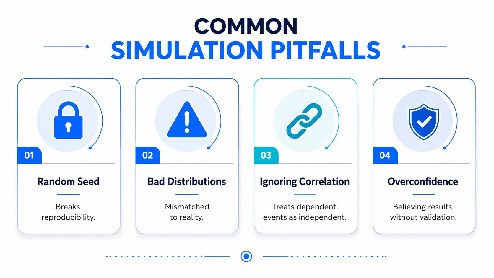
An undisclosed seed makes a result difficult to reproduce. A reviewer may rerun the same code and receive a different output, then mistake normal sampling variation for a logic change. Log the seed, generator, model version, configuration, and input-data snapshot together.

A distribution should have an empirical or domain justification. Plot source histograms, inspect skew and outliers, and compare simulated draws with the observed data. A normal distribution may be convenient, but convenience doesn't make it appropriate for delayed arrivals, service times, or failure intervals that have a long right tail.

Validation rule: Never describe a distribution as realistic until simulated draws have been compared with the behavior they're meant to represent.

Dependence and convergence

Independent draws are not automatically correct. Arrival volume and processing delay may rise together. Missing rows may cluster during a particular upstream failure. If the model samples those variables independently, it can erase the very compound event the team wants to study.

Use scatterplots, time-series analysis, or a documented joint model to inspect dependence. For chain-based or iterative simulations, autocorrelation plots can reveal that adjacent samples aren't independent. The Gelman-Rubin diagnostic can help compare multiple chains when a chain-based method is appropriate, but it isn't a universal convergence test for every independent Monte Carlo harness.

Insufficient iterations produce unstable tail estimates. Plot running estimates, compare batches, and plan trial counts around a target interval width. Report uncertainty intervals alongside point estimates, especially when stakeholders might otherwise treat the central value as a promise.

Avoiding validation overconfidence

A detector validated only on the data used to tune it can appear stronger than it is. Split the data by time or operating condition, validate on a holdout period, and test synthetic scenarios that weren't used to select the threshold. The aim isn't to manufacture a favorable result. It's to discover where the model stops supporting the operational decision.

Building Reliable Simulation Studies

Treat a simulation study like a deployable data product. Before trusting its output, verify that:

• The seed is logged: Record the random generator, seed, model version, and configuration.

• Distributions are justified: Store the source data, fitting method, or domain rationale for every uncertain input.

• Convergence is checked: Compare running estimates and batches against the decision's required precision.

• A baseline exists: Compare the simulation with an analytical estimate, historical replay, or deterministic reference where available.

• Raw trials are stored: Preserve enough output to reproduce summaries, investigate tails, and review unexpected scenarios.

• Inputs are monitored: Rerun the study when upstream data distributions, workload patterns, or pipeline behavior shift.

Choose Monte Carlo when the input distribution is known but the output distribution isn't, when closed-form mathematics is impractical, or when you need empirical confidence intervals instead of a single point estimate. For production teams, that decision belongs alongside broader data observability practices, where observed behavior can inform assumptions and reveal when a simulation no longer reflects reality.

digna provides modular data observability capabilities for anomalies, timeliness, validation, schema changes, and business or platform metrics within your own environment. Visit digna to connect observed pipeline behavior with simulation-based risk analysis and build more defensible reliability decisions.