9 Types of Anomaly Detection Explained
|
10
min read

Most advice about anomaly detection starts with algorithms. That's backwards. Anomaly detection starts with the right definition of normal.
No single method fits every dataset because anomalies come in different forms. A point anomaly is one odd value, like a sudden spike in failed payments. A contextual anomaly only looks wrong in context, like a normal-looking transaction volume that appears at the wrong hour. A collective anomaly is a pattern across multiple records or time steps, such as a delayed batch followed by a catch-up surge. In practice, teams also need to separate univariate problems from multivariate ones, because a single column behaving strangely is very different from several fields drifting together.
That distinction has deep roots. A recent historical survey traces early anomaly thinking in time series back to Bernoulli in 1777, then to Fox's 1972 distinction between anomaly types and Tsay's 1988 expansion, while modern practice still leans on point, contextual, and collective anomalies as core categories (historical survey of time-series anomaly detection). That's still the right starting point for choosing among the main types of anomaly detection.
A practical rule works better than a universal recipe. Use deterministic validation for known conditions. Use statistical or time-series methods when behavior is measurable and recurring. Use machine learning when patterns are complex, multivariate, or shifting too fast for static logic. Platforms such as digna combine statistical methods, machine learning, validation, timeliness, and schema monitoring inside the customer's infrastructure when that operating model matters.
Table of Contents
1. Statistical Baseline Learning
Some teams call this “AI anomaly detection,” but the useful idea is simpler. The system learns what normal behavior looks like from history, then flags deviations from that baseline.
This method works best when a metric has recognizable behavior over time. Transaction counts may rise on weekdays and dip on weekends. Claims data may arrive in predictable waves. Customer support events may spike every morning, then stabilize. A baseline model can absorb those patterns better than a static threshold.
Here's the visual intuition.

What evidence it uses
Baseline learning relies on observed statistical behavior over time. Instead of asking “did this value exceed a fixed limit,” it asks “is this value unusual for this dataset, at this time, under this recent pattern.”
That makes it a practical fit for data observability. A financial team might watch daily transaction volume. A healthcare operations team might monitor admission feeds. A telecom data platform might track late-arriving usage records. In each case, the model learns expected ranges, trends, and recurring variation.
A useful background concept is the distribution of data in anomaly analysis. Teams that understand spread, skew, and expected variation usually tune baselines more effectively.
Practical rule: Pair baseline learning with deterministic checks on high-risk datasets. Learned behavior catches drift. Rules catch known violations.
Where it helps and where it struggles
It helps when “normal” changes over time but still follows a pattern. It struggles when you have too little history, when the process changed last week, or when the metric is mostly noise.
Examples:
Finance: unexpected drift in transaction volume even though no threshold was crossed
Healthcare: unusual shifts in patient activity across facilities
Telecom: abnormal data arrival rates in ingestion pipelines
Common trade-offs:
Strong on interpretability: teams can usually see the expected band and explain why an alert fired
Sensitive to bad training windows: incident periods can contaminate the baseline
Better with supporting controls: validation and timeliness checks improve trust
2. Isolation Forest
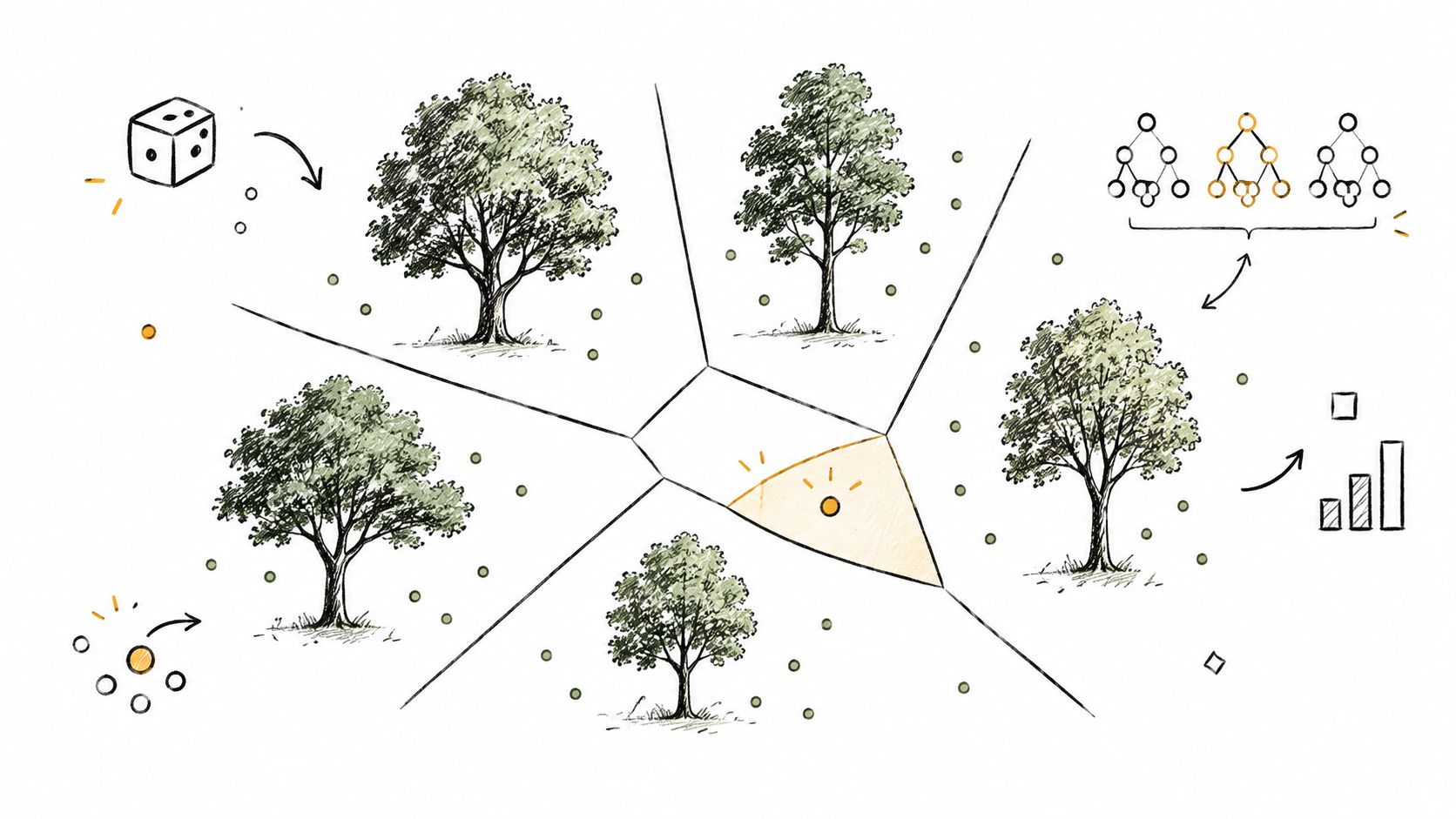
Isolation Forest is a machine learning method that looks strange only until you picture what it's doing. It keeps splitting the data into smaller partitions at random. Points that become isolated quickly are more likely to be anomalies.
That approach makes it useful for high-dimensional data. If you're evaluating many features at once, distance-based methods can become awkward. Isolation Forest avoids some of that complexity by focusing on how easy a point is to separate from the rest.
How it works in practice
You train the model on unlabeled data. It creates many random trees. A normal observation usually takes more splits to isolate because it sits in a dense region. An unusual observation gets separated in fewer steps.
That makes it a reasonable option when you don't have labels and don't want to hand-write rules for every suspicious combination. A bank might score transactions using amount, merchant category, time, geography, and channel. A hospital might analyze combinations of operational measures. A telecom team might monitor network behavior across several dimensions.
If you want to prototype the method hands-on, a Python anomaly detection workflow is a common starting point.
Trade-offs to watch
Isolation Forest can work well on multivariate data, but it isn't magic. Feature choice still matters. So does scaling. If one variable dominates the range, the model may isolate the wrong records for the wrong reason.
Good uses include:
Fraud screening: unusual combinations across many transaction attributes
Operational monitoring: behavior that looks normal on each single metric but odd in combination
Exploration: large unlabeled datasets where you need candidates for review
Start with default parameters, then check real alerts with domain owners. A mathematically unusual point isn't always a business-relevant anomaly.
3. Z-Score and Standard Deviation Methods
If you need a simple answer to “is this value unusually far from the average,” z-score is often the first method to try.
It measures how far a point is from the mean in units of standard deviation. That sounds technical, but the decision logic is straightforward. If the value is far enough away from what's typical, flag it.

Best use case for z-scores
Z-scores are useful when the metric is fairly stable and its distribution is reasonably well behaved. Common baseline techniques for practical statistical anomaly detection include Z-score, IQR, and moving average methods, and teams can combine them through voting or weighted scoring to reduce false alarms and improve detection (practical notes on time-series anomaly detection methods).
That's why z-scores still show up in enterprise monitoring. They're easy to explain. A finance team can flag unusual transaction amounts. A care delivery team can watch outlier vital measurements. A data team can monitor row counts in recurring loads.
If you need to think more carefully about whether mean and spread are the right summary, this guide on how to describe distribution of data is useful context.
Limits and practical adjustments
The weakness is context. A z-score on raw data can miss seasonality, drift, or skewed distributions. A daily sales metric with strong weekday behavior may look anomalous every weekend if you ignore time context.
Use z-scores carefully when:
The metric is stable: row counts, file sizes, durations, or amounts with limited drift
You need transparency: audit or stakeholder review is easier with simple math
You want a baseline benchmark: it's a strong first pass before heavier models
Short practical adjustments:
Use rolling windows: better for changing time-series behavior
Prefer variants when needed: median-based alternatives handle outliers better
Add business rules: a statistically unusual value may still be acceptable operationally
4. Local Outlier Factor
Some anomalies aren't globally extreme. They're only strange relative to nearby data. That's where Local Outlier Factor, or LOF, becomes useful.
LOF compares the local density of a point to the density of its neighbors. If the point sits in a thinner region than the records around it, the method treats it as suspicious. This makes it good for clustered data where “normal” has several modes.
Why density matters
Think about customer usage in telecom. Heavy users, casual users, and enterprise accounts may all form separate groups. A record might look normal compared with the whole population but still look odd inside its own cluster. LOF is built for that kind of contextual comparison.
The same logic helps in platform monitoring. A set of jobs may all run within one latency band, while another pipeline family runs in a different band. LOF can catch a task that's abnormal for its peer group even if it doesn't look large in absolute terms.
Practical fit and trade-offs
LOF is strongest when neighborhoods are meaningful. It weakens when dimensions multiply and everything becomes sparse. In high-dimensional data, nearest-neighbor relationships can become less informative.
Useful scenarios:
Telecommunications: unusual customer behavior inside similar usage cohorts
Data platforms: anomalous jobs relative to comparable jobs
Healthcare operations: records that don't fit nearby operational patterns
Points to remember:
Choose neighborhood size carefully: too small and alerts become twitchy, too large and local context disappears
Scale features first: density comparisons break when one feature dominates
Use review loops: LOF often finds subtle cases that need business interpretation
LOF usually works better as part of a stack than as a lone detector. Pair it with a simple statistical screen or a deterministic rule to cut review noise.
5. Autoencoder Neural Networks
Autoencoders belong to the reconstruction family. Instead of setting explicit limits or measuring density, they learn to compress and rebuild normal data. When reconstruction goes badly, the input may be anomalous.
That idea is powerful when the pattern is complex and nonlinear. It's also the point where anomaly detection becomes harder to explain to nontechnical stakeholders.
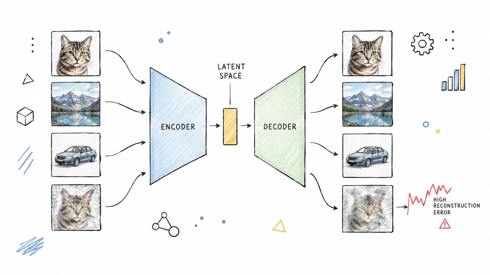
Where reconstruction helps
Autoencoders are useful when normal behavior depends on many interacting variables and simple boundaries won't capture it. A finance team might score complex pricing behavior. A healthcare team might monitor combinations from multiple devices or sensors. A telecom team might evaluate traffic signatures that don't separate cleanly with linear methods.
In broad surveys, anomaly detection methods are often grouped into statistical approaches, classical machine learning approaches, and neural-network-based methods (survey of statistical, machine learning, and deep learning methods). Autoencoders sit firmly in that third group.
For time-based behavior, they often appear in broader time-series anomaly detection workflows, especially when relationships across signals matter more than any single metric.
The trade-offs are real
Autoencoders can capture patterns that simpler methods miss. They also need cleaner training data, more tuning, and stronger operational discipline. If the model learns corrupted “normal,” reconstruction error becomes less meaningful.
Use them when:
Patterns are complex: nonlinear interactions matter
Labeled anomalies are scarce: reconstruction doesn't require many examples of failure
You can support the model: training, retraining, and threshold review need ownership
Neural methods often find valuable anomalies, but they rarely replace simpler controls. Teams still need explainable checks for incident review and audit conversations.
6. One-Class SVM Support Vector Machine
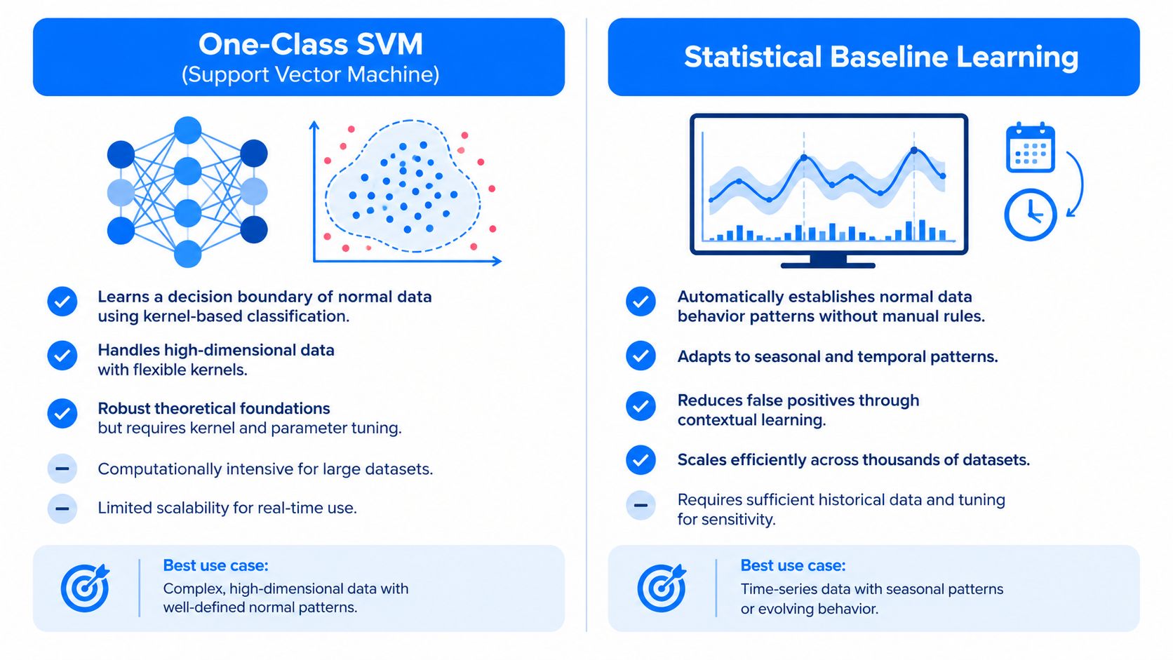
One-Class SVM tries to learn the boundary around normal data. Anything outside that learned boundary is treated as unusual.
That makes it conceptually different from Isolation Forest. Isolation Forest asks how easy a point is to separate. One-Class SVM asks whether the point falls inside the accepted region of normal behavior.
When boundary learning makes sense
This method is useful when normal records form a coherent shape, even if that shape isn't linear. Kernel functions let the model draw more flexible boundaries, which can help with multivariate patterns.
Examples include:
Financial services: transactions that fall outside normal customer behavior
Healthcare: unusual clinical profiles across several measurements
Customer analytics: account activity patterns that drift beyond known norms
The main challenge is sensitivity. One-Class SVM can react strongly to feature scaling, parameter choices, and noisy training data. On large datasets it can also become computationally expensive compared with lighter methods.
What teams should expect
One-Class SVM is often a good choice for medium-sized, structured datasets where “normal class only” learning fits the business problem. It's less attractive when you need easy explainability or low-maintenance production behavior.
Helpful operating habits:
Normalize inputs: this is rarely optional
Keep features meaningful: weak features distort the boundary
Retrain after process changes: new products, channels, or workflows can move the normal region
If you need a model that's easier to discuss with auditors or operations managers, deterministic validation or statistical baselines usually win.
7. Seasonal Decomposition and ARIMA
Time changes everything in anomaly detection. A value can look wrong only because it appeared at the wrong hour, on the wrong day, or after the wrong sequence. Seasonal decomposition and ARIMA are built for that problem.
These methods use temporal expectation as evidence. They ask what should happen next, given the history of the series.
The benchmarking environment shows why careful method selection matters. ADBench evaluated 30 anomaly detection algorithms on 57 datasets, and the UCR Time Series Anomaly Archive provides 250 curated time series for research, reinforcing that algorithm choice depends heavily on dataset characteristics (ADBench benchmark and UCR archive overview).
What they look for
Seasonal decomposition separates a series into trend, seasonality, and residual behavior. ARIMA models temporal dependence directly. Both are useful when the anomaly is not just “high” or “low,” but “unexpected for this point in time.”
That matters in real operations. A nightly batch load that doesn't arrive on schedule is a timeliness issue. A customer activity spike on a holiday might be normal if seasonality and event context are modeled correctly. A revenue dip on a quiet weekend may not deserve escalation.
The method family is especially relevant for collective and subsequence anomalies. A recent survey notes that many production incidents are not isolated points but collective or subsequence anomalies, and it highlights the practical gap in method choice for cases like delayed loads, schema drift, and multi-signal pipeline behavior (survey on systemic shift detection and observability data). If you work on data delivery monitoring, that gap will sound familiar.
A useful implementation reference is this guide to detecting anomalies in time series.
Good fit for data observability
These methods are often the right answer for:
Missing or late loads: expected arrival windows matter more than raw values
Seasonal business metrics: daily, weekly, or monthly patterns drive normal behavior
Drift in recurring processes: gradual departures from historical timing or volume
A delayed pipeline is often a collective anomaly, not a point anomaly. Time-aware methods catch that sooner than static thresholds.
8. Mahalanobis Distance
Mahalanobis distance is one of the most useful multivariate statistical tools that many teams skip. It measures how far a point is from the center of the data while accounting for scale and correlation.
That last part matters. If two variables usually move together, a record can look perfectly normal on each individual column and still be strange as a combination.
Why correlation changes the answer
Suppose revenue growth, margin, and debt ratio usually follow a known relationship for a segment. A company record with ordinary values on each metric may still violate the usual multivariate pattern. Mahalanobis distance can surface that mismatch more effectively than simple Euclidean distance.
This makes it useful in finance, clinical operations, and data quality monitoring. A healthcare record may show individually plausible values that create an implausible profile when combined. A data platform may observe quality metrics that are acceptable alone but suspicious together.
When to use it
Mahalanobis distance is a strong middle ground between simple statistics and full machine learning. It remains interpretable, but it handles multivariate structure better than per-column thresholds.
It works best when:
Variables are correlated: covariance carries useful information
You need explainable multivariate checks: analysts can inspect which relationships shifted
The data is structured: stable metrics often suit it better than raw event streams
Covariance estimates can become unstable in noisy or high-dimensional settings. Segmented covariance estimation and segmentation often improve reliability.
9. Rule-Based and Deterministic Validation
The most neglected advice in anomaly detection is this. If the business already knows a condition is unacceptable, don't train a model to rediscover it.
Rule-based validation uses explicit logic. Required fields must be populated. Reference values must match approved lists. Dates must follow sequence constraints. Regulatory conditions must hold exactly. This is not “old school” monitoring. It's the clearest form of evidence you can have.
The strongest kind of signal
Rules use explicit business knowledge rather than inferred patterns. If a healthcare file must include mandatory identifiers, there's no benefit in asking a statistical model whether missing identifiers look unusual. They are invalid. If a financial process requires amounts to stay within a defined policy range, a deterministic control is the primary check.
This is why rule-based methods remain essential in regulated environments and critical reporting workflows. They give teams complete auditability and stable operational behavior.
Examples:
digna Data Validation: record-level checks against business rules
Financial services: controls tied to policy or regulatory constraints
Healthcare: mandatory field completeness and logical consistency
Public sector: audit-ready enforcement of required data conditions
Where rules end
Rules are precise, but they only catch what someone thought to define. They won't detect an unusual customer mix, a subtle metric drift, or a shifting baseline in arrival timing.
Recent reviews emphasize that practical anomaly detection evaluation still needs better guidance under privacy, deployment, explainability, and operational constraints, while observability research continues to highlight the challenge of reducing noise across logs, traces, and metrics with trusted automation (review of operational, explainable, and deployment-aware anomaly detection). Deterministic validation helps with trust because teams can see the exact condition that failed.
Use rules for:
Known business requirements
Compliance and audit controls
High-risk fields and records
Clear escalation paths
Comparison of 9 Anomaly Detection Methods
Method | 🔄 Implementation complexity | ⚡ Resource requirements | 📊 Expected outcomes | 💡 Ideal use cases | ⭐ Key advantages |
|---|---|---|---|---|---|
Statistical Baseline Learning | Moderate, automated setup, sensitivity tuning | Low–Medium, needs historical data, modest compute | Context-aware anomaly detection with reduced false positives | Continuous KPI/data-quality monitoring, seasonal metrics | Auto-adapts to trends and seasonality; scalable; fast time-to-value |
Isolation Forest | Moderate, train trees and tune params | Low–Medium, efficient for large/high-dim data | Strong multivariate anomaly detection in high dimensions | Fraud detection, high-dimensional operational datasets | Efficient, robust to irrelevant features, no distance metric needed |
Z-Score & Standard Deviation | Low, simple statistical calculations | Minimal, negligible compute | Fast, interpretable single-metric outlier flags | Row counts, single-metric thresholds, first-line monitoring | Extremely fast, transparent, easy to audit and implement |
Local Outlier Factor (LOF) | Moderate–High, neighbor selection and distance metric | Medium–High, costly for large samples or high dimensions | Detects local density deviations and cluster-specific outliers | Datasets with varying densities or cluster-dependent anomalies | Captures local context; no global distribution assumption |
Autoencoder Neural Networks | High, architecture design and hyperparameter tuning | High, GPUs, large labeled/clean training set helpful | Detects complex non-linear anomalies via reconstruction error | Complex high-dimensional patterns, multi-sensor or temporal data | Models non-linear relationships; scalable to complex feature sets |
One-Class SVM | High, kernel selection and parameter tuning | Medium–High, memory & compute rise with data size | Boundary-based detection; sensitive to scaling and kernels | Cohesive-normal-region datasets where anomalies lie outside | Flexible decision boundaries with strong theoretical basis |
Seasonal Decomposition & ARIMA | Moderate, seasonal/ARIMA parameter selection | Low–Medium, needs long historical series | Interpretable trend/seasonality components and forecasted anomalies | Time-series with strong seasonality, pipeline timeliness | Designed for temporal data; clear decomposition and forecasts |
Mahalanobis Distance | Low–Moderate, covariance estimation and inversion | Low–Medium, needs sufficient samples per dimension | Multivariate outlier scores accounting for correlations | Correlated multivariate quality checks and monitoring | Accounts for covariance and scale; effective for correlated variables |
Rule-Based & Deterministic Validation | High, manual rule authoring & maintenance | Medium, human effort; low compute | Deterministic pass/fail results with full auditability | Regulatory/compliance checks and critical business rules | Fully transparent, auditable, exact enforcement of business logic |
Choose the Method That Matches the Signal
The most practical way to understand the types of anomaly detection is to stop treating them as rival camps. They are different ways of gathering evidence.
Use z-scores when a metric is simple, stable, and easy to summarize with mean and spread. Use baseline learning when dataset behavior changes over time but still forms an expected pattern. Use seasonal decomposition or ARIMA when timing, trend, and recurrence matter, especially for missing loads, delivery delays, and business activity with daily or weekly rhythm. Use LOF and Mahalanobis distance when context comes from neighboring points or correlated variables. Use Isolation Forest, One-Class SVM, or autoencoders when the data is unlabeled, multivariate, and too complex for static logic.
The broader method area reflects that diversity. Time-series anomaly detection is commonly classified into unsupervised, supervised, and semi-supervised learning types, and the same literature groups methods into forecasting, reconstruction, distance, encoding, neighborhood, and probabilistic families (VLDB overview of time-series anomaly detection families). That's a helpful reminder that algorithm choice should start with the signal, not with a favorite model.
The market direction also points toward operational combinations rather than isolated tools. One industry forecast projects the anomaly detection market to grow from USD 4.28 billion in 2024 to USD 9.25 billion by 2032, and attributes 2025 adoption leadership to software with an 81.6% share and cloud deployment with a 72.8% share (anomaly detection market forecast). That doesn't mean every team should rush to a cloud-only stack. It does show that scalable, production-oriented anomaly detection has moved into mainstream enterprise operations.
For data observability, the strongest setup usually combines methods. A deterministic rule can reject impossible records. A baseline model can detect gradual drift in row counts or values. A timeliness detector can spot delayed loads. A schema monitor can catch structural changes before downstream consumers fail. That layered design matches how incidents happen. Few production failures announce themselves through one perfect signal.
digna is a relevant example of that combined approach. Its platform runs inside the customer's own environment and brings together AI-driven anomaly detection, record-level validation, timeliness monitoring, schema tracking, business and platform metric monitoring, and in-database execution. That combination matters for teams that need both adaptive detection and controlled, auditable enforcement.
Use this checklist before you choose a method:
Define the anomaly clearly: is it a point, contextual, collective, univariate, or multivariate problem?
Confirm the data history: do you have enough clean history to learn normal behavior?
Measure false positives: who will review alerts, and what level of noise is acceptable?
Assign response ownership: which team investigates drift, failed rules, or delivery delays?
Review after process change: retrain, retune, or rewrite controls when products, pipelines, or schedules change
The right method is the one that fits the signal, the data, and the operational reality around both.
digna gives data teams a modular way to apply these anomaly detection approaches in production, from AI-driven baseline learning to deterministic validation, timeliness monitoring, and schema tracking. Because it runs inside the customer's own environment and executes checks in-database, it fits teams that need observability with strong control over data movement and review workflows. If that matches your setup, visit digna.
Choosing a method is the easy half; keeping it calibrated as the data shifts is the work, and that is where continuous data quality monitoring earns its place.
Frequently asked questions
Where should anomaly detection actually start?
With the right definition of normal, not with algorithms. Most advice starts from the method, which is backwards: the same deviation can be an incident in one dataset and expected seasonality in another, and no model settles that question for you.
What's the difference between statistical baselines and isolation forests?
Statistical baseline learning models expected behaviour from history and flags departures from it. Isolation forests instead isolate points that are easy to separate from the rest, which scales well on high-dimensional data but gives you less intuition about why a point was flagged.
When should you use z-scores rather than density methods?
Z-scores suit roughly normal, single-variable distributions where deviation from the mean is meaningful. Local Outlier Factor earns its place when density matters — when a point is normal globally but unusual relative to its immediate neighbours, which z-scores cannot see.
Which methods suit time-series data?
Seasonal decomposition and ARIMA, because they separate trend and seasonality from the residual and look for deviation in what remains. That fits data observability well, where a Monday spike is routine and the same spike on a Wednesday is not.
Do rule-based checks still matter alongside ML?
Yes — deterministic validation is the strongest kind of signal, because it is explainable and auditable in a way a model score is not. Rules end where the unknown unknowns begin, which is exactly where behavioural methods take over.