Monte Carlo Simulation for Beginners: A Hands-On Guide

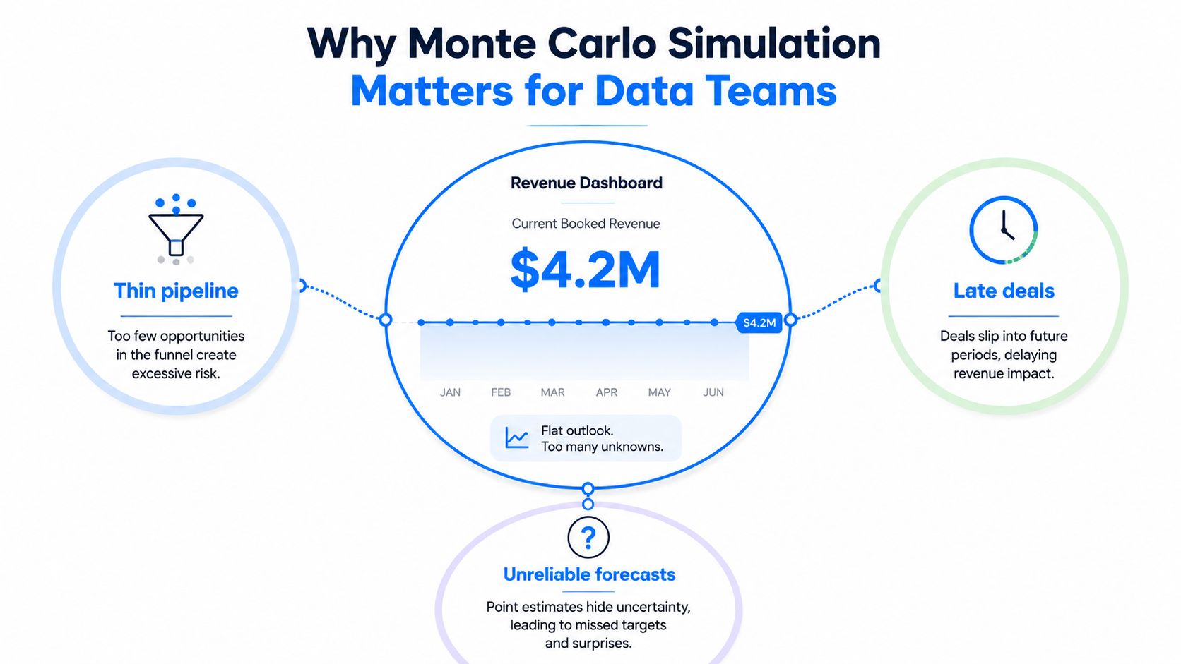
Your quarterly revenue dashboard has shown the same $4.2M line for three weeks. The chart looks reassuring, but the deal pipeline underneath is thin, several opportunities are late, and forecast confidence is poor. A single number is hiding a wide range of plausible outcomes.

That's the kind of problem Monte Carlo simulation helps data teams solve. Instead of forcing uncertain inputs into one deterministic forecast, you repeatedly sample realistic possibilities and examine the distribution of resulting metrics. The method is useful for learning how uncertainty affects revenue, pipeline delivery, data availability, and the KPIs built on top of them.

Table of Contents

• Why Monte Carlo Simulation Matters for Data Teams

  • From dashboard certainty to decision range

• The Core Idea Behind Monte Carlo Simulation

  • Estimating pi with random points

  • The three building blocks

• Building Your First Simulation in Python

  • Reading the output correctly

• Practical Use Cases for Estimation and Risk

  • Revenue uncertainty

  • Pipeline completion risk

  • Data availability gaps

• How Many Iterations You Need

  • A practical convergence check

• Common Pitfalls and Validation Checks

  • Match distributions to the data

  • Preserve relationships between inputs

  • Make runs reproducible

  • Validate before trusting the histogram

• Connecting Simulation to Data Quality and Observability

  • A production workflow

Why Monte Carlo Simulation Matters for Data Teams

A point estimate is convenient because it's easy to display and discuss. It's also incomplete. When a dashboard reports one revenue figure, one pipeline completion time, or one expected null rate, the calculation may have compressed uncertain inputs into fixed assumptions long before the result reached a stakeholder.

Monte Carlo simulation restores that missing variation. Each run represents one plausible state of the system. A revenue run might include fewer successful deals, later close dates, or different deal values. A pipeline run might combine a larger input volume with resource contention. After many runs, the team can examine not just the central estimate, but also the lower and upper portions of the outcome distribution.

From dashboard certainty to decision range

Suppose the revenue dashboard remains flat because the reporting query uses the current forecast total. That total says nothing about how sensitive the result is to late deals or unreliable opportunity stages. A simulation can produce a range that answers more useful questions:

• Revenue exposure: How low could recognized revenue plausibly fall if uncertain deals slip?

• Planning confidence: How much of the reported forecast depends on a small number of opportunities?

• Operational response: Should finance adjust hiring plans, or should sales operations improve pipeline data first?

The same reasoning applies to data engineering. A job may have a nominal completion time, but row counts, upstream delays, and warehouse contention create operational uncertainty. Simulating those inputs helps the team estimate the risk of missing an SLA rather than relying on an average runtime.

Practical rule: Report the forecast and the uncertainty around it. Stakeholders can act on a range when they understand what drives the range.

This approach complements data observability practices, where teams monitor whether data arrived, changed, or violated expectations. Monitoring tells you what is happening. Simulation helps estimate what the observed conditions could do to downstream decisions.

The Core Idea Behind Monte Carlo Simulation

Monte Carlo simulation is built from a simple loop: define a system, generate random inputs, calculate an outcome, and repeat. The result isn't a special kind of random number. It's a collection of outcomes that approximates the behavior of an uncertain system.

The classic pi example makes the logic visible without code.

Estimating pi with random points

Start with a square and draw a circle inside it so the circle touches the square's boundaries. The square defines the domain. Now drop points randomly across the square, giving every location an equal chance of receiving a point.

For each point, check whether it falls inside the circle. You can do that by comparing its distance from the center with the circle's radius. The points inside the circle form a sample of the circle's area, while all points together represent the square's area.

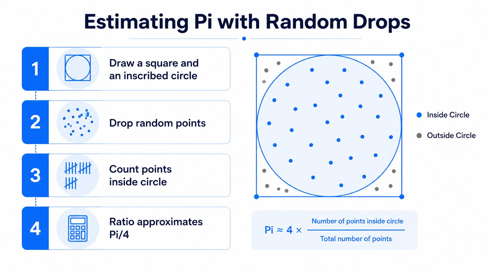
The aggregation rule is the important part. Divide the number of points inside the circle by the total number of points. That ratio approximates the circle's area divided by the square's area, which is π divided by four. Multiply the ratio by four, and you have an estimate of π.

The estimate won't be exact after a small number of trials. Random clustering creates noise. As you repeat the experiment, the estimate generally settles around the mathematical value, although individual runs can still differ.

The three building blocks

A beginner-friendly way to think about a simulation is to separate its structure into three pieces:

1. Domain: Define the possible input space, such as the square containing the circle.

2. Sampling process: Draw random values according to a specified distribution, such as uniform points across the square.

3. Aggregation rule: Turn each trial into an output, then summarize the collection with a metric such as a ratio, mean, or percentile.

The same pattern appears in enterprise data work. The domain might be plausible deal values, the sampling process might draw from a triangular distribution, and the aggregation rule might sum expected revenue across opportunities. Understanding how distributions describe data is essential because the distribution determines which possibilities the simulation considers common, rare, or impossible.

Building Your First Simulation in Python

The first Python simulation should stay small enough to inspect. The standard library gives you everything needed for the pi example: random generates samples, and math provides the reference value for calculating error.

The script below defines the inputs, fixes a seed for repeatability, counts points inside a unit circle, and prints progress at useful milestones.

import math
import random

TRIALS = 100_000
SEED = 42
random.seed(SEED)

inside = 0
milestones = {1_000, 10_000, 100_000}

for trial in range(1, TRIALS + 1):
    x = random.uniform(-1, 1)
    y = random.uniform(-1, 1)

    if x * x + y * y <= 1:
        inside += 1

    if trial in milestones:
        estimate = 4 * inside / trial
        error = abs(estimate - math.pi)
        print(
            f"Trials: {trial:,}, "
            f"estimate: {estimate:.6f}, "
            f"absolute error: {error:.6f}"
        )

import math
import random

TRIALS = 100_000
SEED = 42
random.seed(SEED)

inside = 0
milestones = {1_000, 10_000, 100_000}

for trial in range(1, TRIALS + 1):
    x = random.uniform(-1, 1)
    y = random.uniform(-1, 1)

    if x * x + y * y <= 1:
        inside += 1

    if trial in milestones:
        estimate = 4 * inside / trial
        error = abs(estimate - math.pi)
        print(
            f"Trials: {trial:,}, "
            f"estimate: {estimate:.6f}, "
            f"absolute error: {error:.6f}"
        )

import math
import random

TRIALS = 100_000
SEED = 42
random.seed(SEED)

inside = 0
milestones = {1_000, 10_000, 100_000}

for trial in range(1, TRIALS + 1):
    x = random.uniform(-1, 1)
    y = random.uniform(-1, 1)

    if x * x + y * y <= 1:
        inside += 1

    if trial in milestones:
        estimate = 4 * inside / trial
        error = abs(estimate - math.pi)
        print(
            f"Trials: {trial:,}, "
            f"estimate: {estimate:.6f}, "
            f"absolute error: {error:.6f}"
        )

The inputs have distinct jobs. TRIALS controls how long the experiment runs, while SEED makes the random sequence reproducible. Reproducibility matters in data engineering because you need to distinguish a model change from ordinary sampling variation.

Reading the output correctly

At each milestone, the script calculates the current estimate and its absolute error from the true value of π. The early estimate may move noticeably, while later estimates often appear steadier. That pattern is useful, but don't treat the final printed number as the whole result.

A stronger version stores each milestone estimate and plots it against the trial count. Add a horizontal reference line at math.pi, then inspect whether the estimate is tightening around that line. The chart shows convergence directly, which is more informative than comparing two isolated outputs.

The spread across independent runs is part of the signal. A single reproducible result is useful for debugging, but it doesn't describe the uncertainty of the method.

For production data work, the same structure can support Python-based data anomaly detection. Replace the random coordinates with sampled operational inputs, replace the circle test with your business or pipeline logic, and preserve the output distribution for review.

Practical Use Cases for Estimation and Risk

The pi example uses a geometric relationship, but enterprise simulations usually propagate uncertainty through a business or pipeline model. The loop remains familiar: sample inputs, apply the model, save the result, and summarize the output.

Revenue uncertainty

Consider a quarterly portfolio containing opportunities with uncertain close values. For each deal, use a triangular distribution with a minimum, most likely value, and maximum. The minimum can represent a conservative outcome, the most likely value can reflect the current sales assessment, and the maximum can represent the strongest plausible close.

One simulation run samples one value for every deal and adds those values together. Repeating the process creates a distribution of portfolio revenue. The mean provides a central estimate, while selected percentiles provide a range for planning. The value comes from showing how uncertainty compounds across the portfolio, especially when a small group of deals contributes heavily to the forecast.

This same style of probabilistic forecasting appears in other decision contexts. Readers who work with event probabilities may find the discussion of Monte Carlo for prediction market traders useful because it applies repeated sampling to uncertain outcomes rather than relying on a single deterministic forecast.

Pipeline completion risk

For an ETL job, sample uncertain row counts, processing rates, upstream arrival times, and resource contention. The aggregation logic can calculate the expected finish time for each run. The decision output is whether that finish time falls before the SLA window.

The result can guide capacity planning. If the simulated finish-time distribution frequently crosses the deadline, the team has evidence to investigate partitioning, workload scheduling, upstream dependencies, or the SLA itself.

Data availability gaps

A data team can also simulate missingness across source tables. Sample null rates or missing-load conditions from observed operational behavior, apply those conditions to the KPI calculation, and record the resulting metric. The output distribution shows how much the KPI could move when source completeness changes.

The code structure barely changes between these examples. The important work happens in the input model and aggregation logic. If those assumptions don't reflect how the business or pipeline behaves, more runs won't repair the model.

Present results as ranges tied to decisions. “The KPI may move across a broad plausible interval when source completeness deteriorates” gives an executive a reason to fund remediation. A lone forecast number hides that operational choice.

How Many Iterations You Need

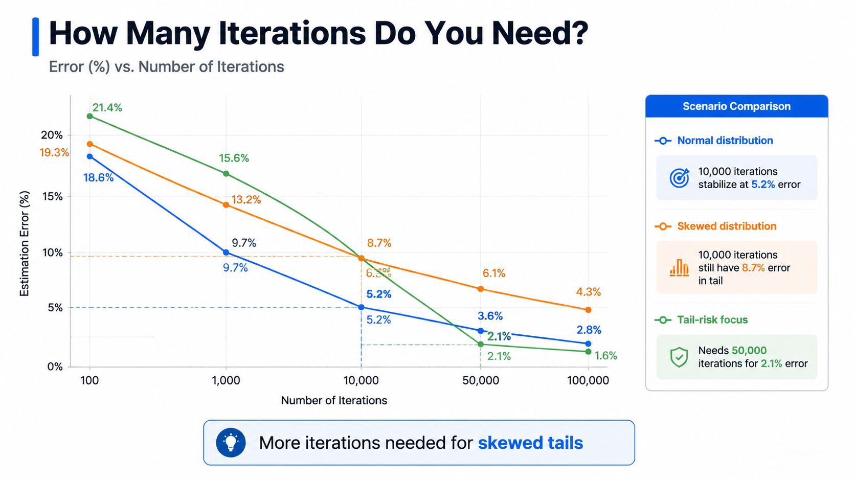
10,000 iterations is not a universal answer. One practical guide recommends 10,000 iterations for many business applications and suggests checking whether key outputs change by less than 1% when increasing the run count from 10,000 to 20,000. It contrasts that recommendation with AWS guidance suggesting sample sizes in the range of 100,000 for accuracy. Read the practical convergence discussion for that comparison.

The required run count depends on the decision and the output being measured. A mean may stabilize while a 95th percentile remains noisy. Skewed or heavy-tailed inputs need more runs than compact, balanced inputs, while correlated variables can reduce the effective information provided by each sample.

AWS guidance favors stopping when the simulation meets an error tolerance, including the standard error of the mean, instead of selecting a fixed count in advance. That approach also fits data engineering work, where a KPI estimate and an SLA-risk percentile may need different precision. For background on related statistical methods for data analysis, connect the convergence check to the metric's intended use.

A practical convergence check

Record the running mean and lower and upper tail percentiles at regular checkpoints. The following pattern checks every 500 iterations, then gives you values to plot and compare.

checkpoints = []
results = []

for trial in range(1, total_trials + 1):
    result = run_model()
    results.append(result)

    if trial % 500 == 0:
        ordered = sorted(results)
        mean = sum(results) / len(results)
        lower = ordered[int(0.05 * len(ordered))]
        upper = ordered[int(0.95 * len(ordered))]

        checkpoints.append((trial, mean, lower, upper))

checkpoints = []
results = []

for trial in range(1, total_trials + 1):
    result = run_model()
    results.append(result)

    if trial % 500 == 0:
        ordered = sorted(results)
        mean = sum(results) / len(results)
        lower = ordered[int(0.05 * len(ordered))]
        upper = ordered[int(0.95 * len(ordered))]

        checkpoints.append((trial, mean, lower, upper))

checkpoints = []
results = []

for trial in range(1, total_trials + 1):
    result = run_model()
    results.append(result)

    if trial % 500 == 0:
        ordered = sorted(results)
        mean = sum(results) / len(results)
        lower = ordered[int(0.05 * len(ordered))]
        upper = ordered[int(0.95 * len(ordered))]

        checkpoints.append((trial, mean, lower, upper))

Plot the three recorded series. Increase the run count until the running mean and both tail lines are stable enough for the decision, such as a capacity choice, financial commitment, or SLA review.

A useful internal tolerance can be a relative standard error under 1–2% for point estimates and under 5% for tail percentiles. These are operating targets, not mathematical guarantees. Document why they fit the use case, particularly when the output affects production planning or data quality remediation.

Common Pitfalls and Validation Checks

A simulation can produce a polished histogram and still be wrong. Most failures begin before the random loop, in the assumptions that define the inputs and relationships.

Match distributions to the data

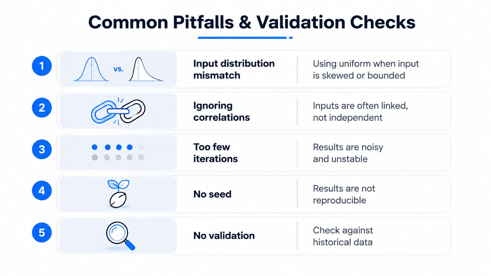
Uniform sampling is attractive because it's simple, but it says every value in the range is equally plausible. That rarely fits a skewed business input. Revenue deals often need triangular or PERT-style assumptions, while positive operational measures may need a right-skewed distribution.

Use historical observations where available. If history is sparse, record the reasoning behind the minimum, most likely, and maximum values instead of presenting expert judgment as measured fact.

Preserve relationships between inputs

Independent sampling can overstate diversification. Two revenue opportunities may depend on the same customer budget, and two pipeline stages may compete for the same warehouse resources.

Model dependence explicitly. A covariance matrix with a Cholesky decomposition can generate correlated samples, while deterministic streams can preserve known relationships. Validate the simulated correlation against the relationship you intended to represent.

Make runs reproducible

Without a seed, a rerun changes the random sequence. That makes debugging harder and can create unnecessary disagreement between development and production results.

Set a seed during testing, record it with the run metadata, and use controlled random streams when parallel workers execute simulations. For production reporting, distinguish a reproducible audit run from a broader set of independent runs used to assess sampling variability.

Validate before trusting the histogram

Start with a simple case whose answer you can calculate analytically. The pi example provides that kind of check. In a revenue model, test a deliberately simplified portfolio where the expected result is easy to derive. In a pipeline model, use fixed inputs first, then introduce variability one input at a time.

Validation principle: A simulation should earn trust through comparison, not through visual polish.

Finally, don't publish only the mean. Include the selected interval, the input assumptions, the seed or run configuration, and the convergence evidence. A stakeholder needs to know what the model says and how much confidence to place in it.

Before sharing a result, check:

• Input fit: Do the distributions reflect observed behavior and valid bounds?

• Dependencies: Have shared drivers and correlations been modeled?

• Reproducibility: Can another engineer rerun the same configuration?

• Convergence: Do the mean and relevant percentiles stabilize?

• Sanity check: Does a simplified version match an analytical or historical expectation?

• Communication: Are ranges, assumptions, and limitations visible beside the point estimate?

Connecting Simulation to Data Quality and Observability

Monte Carlo simulation doesn't replace monitoring. A data observability system can surface missing records, freshness failures, unusual volumes, validation errors, and schema changes as they occur. Simulation answers a different question: what downstream uncertainty could those conditions introduce into a KPI, dashboard, or machine-learning feature?

Consider a freshness alert on a source table. The monitoring layer records the delay and the affected dataset. The data team can then parameterize a simulation with observed delivery behavior, completeness patterns, and the KPI's dependency logic. Each run estimates a plausible KPI outcome under those conditions, producing a risk range that helps the team prioritize remediation.

That prioritization is more useful than counting alerts. A minor anomaly in an isolated table may deserve less immediate attention than a moderate completeness issue affecting a regulatory metric or executive dashboard. The simulation connects the technical event to business exposure.

A production workflow

A practical implementation can follow this sequence:

1. Instrument the pipeline: Capture freshness, volume, null rates, validation failures, and schema changes.

2. Create model inputs: Convert observed quality behavior into distributions with explicit bounds and assumptions.

3. Run the KPI model: Sample the quality inputs and calculate the affected metric for each trial.

4. Store the result: Save the run configuration, convergence information, output range, and timestamp beside the dashboard.

5. Review the drivers: Use sensitivity analysis to identify which quality condition contributes most to metric uncertainty.

The Monte Carlo methods for better data observability approach connects these probabilistic forecasts with operational quality signals. digna can combine data behavior monitoring, validation, timeliness tracking, anomaly detection, and schema monitoring inside the customer's environment, allowing teams to retain data in place while relating observed quality conditions to metric risk.

Start with one KPI that stakeholders already question. Define its upstream dependencies, collect the quality signals that affect it, and run a controlled simulation with documented assumptions. Once the output proves useful in incident review, add it to the dashboard so stakeholders see both the current data status and the uncertainty surrounding the metric.

digna helps data teams monitor quality, timeliness, anomalies, validation results, schema changes, and business metrics in their own environment, creating the operational inputs needed for uncertainty-aware analysis. Visit digna to explore how the platform can connect data observability signals with Monte Carlo methods for more defensible analytics.