Monte Carlo Simulation Tutorial for Data Engineers in 2026

You've probably seen this failure already. A dashboard reports a clean revenue figure, while the pipeline that produced it arrived late, processed an unusual volume, or dropped records. The number looks precise because the dashboard shows one value, but the platform engineer still needs to answer the harder question: how much confidence should the business place in it, and how likely is the pipeline to miss its delivery commitment?

A Monte Carlo simulation replaces that false precision with a distribution of plausible outcomes. In a production data platform, the useful result isn't a colorful histogram by itself. It's a defensible estimate of delivery risk, metric uncertainty, anomaly-detector performance, or operational capacity, backed by validated assumptions and convergence checks.

Table of Contents

• What Monte Carlo Simulation Actually Solves in a Data Platform

  • The historical method and the engineering use case

• Picking the Right Distributions for Real Inputs

  • Fit a model, then challenge it

  • Distribution Selection Cheat Sheet for Data Platform Inputs

• Building Your First Simulation in Python

  • Model and vectorized driver

  • Reporting the result

• Variance Reduction and Convergence Diagnostics

  • Diagnostics that belong in the run

• Common Pitfalls That Break Production Simulations

  • Read the failure in the dashboard

  • Percentiles need uncertainty too

• Practical Use Cases for Data Engineers

  • Uncertainty around business metrics

  • SLA breach probability for data delivery

  • Synthetic anomaly data for detector benchmarking

• Production Checklist for Shipping a Monte Carlo Model

  • Reproducibility and governance

  • Runtime controls

What Monte Carlo Simulation Actually Solves in a Data Platform

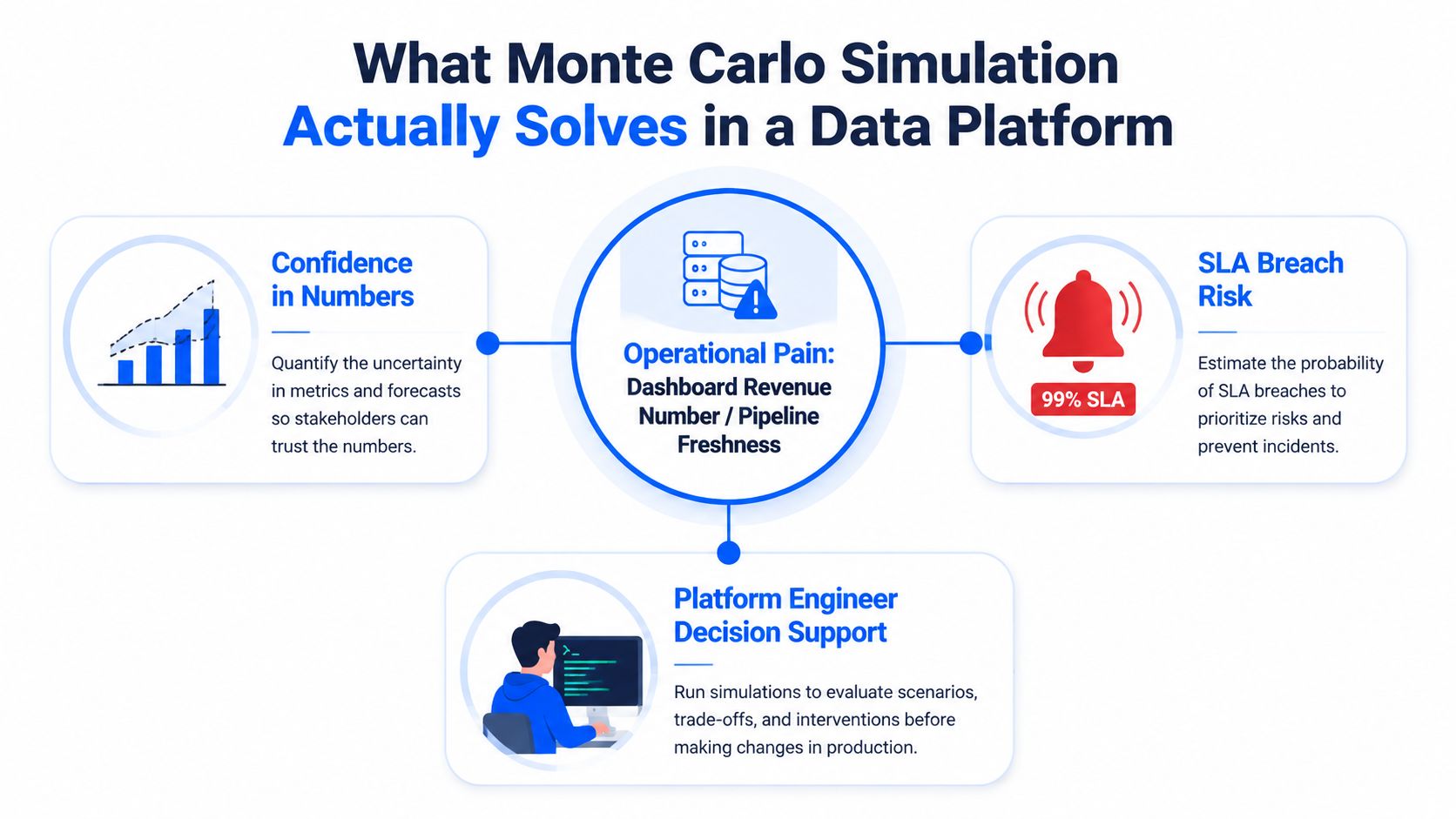
A deterministic pipeline forecast might say that a nightly job will finish at a particular time. That estimate usually hides variation in source volume, upstream delays, warehouse contention, partition counts, and stage duration. If the job must land by 06:00, the operational question isn't “what's the average completion time?” It's “what portion of plausible runs finish late?”

Monte Carlo simulation answers that question through repeated random sampling. You represent uncertain inputs with distributions, draw a plausible value for each input, run the pipeline model, and record the result. Repeating that process produces an outcome distribution rather than a single point estimate. The technique is broadly defined as a repeated-random-sampling method for numerical analysis, and statistics teaching research describes it as a computer-driven experiment that generates plausible sample data from known parameters, with applications ranging from particle physics and molecular modeling to traffic, environmental science, and financial simulation (statistics teaching research).

The historical method and the engineering use case

The modern method emerged at Los Alamos in the mid-1940s and was first fully automated on an ENIAC computer in the spring of 1948. Historical accounts identify Stanisław Ulam as the inventor of the modern version, with John von Neumann, Nicholas Metropolis, and others developing early computerized calculations for nuclear-weapon core simulation (history of the Monte Carlo method).

The origin matters because it highlights the method's purpose. Monte Carlo was built for systems that were too complex for direct calculation. Data platforms have a similar problem, although the sources of uncertainty are different. Ingestion latency, workload size, retries, concurrency, and freshness behavior interact in ways that a single average cannot describe.

For prediction-market-style thinking about uncertain outcomes, prediction market Monte Carlo strategies provide useful conceptual context. For data teams, the practical extension is to connect the simulation output to observability rather than leave it in a notebook. A useful overview is digna's discussion of Monte Carlo methods for better data observability, particularly when teams need to turn probabilistic results into recurring monitoring signals.

Production rule: A simulation becomes trustworthy only when its input assumptions, convergence behavior, and operational decision are all visible.

Picking the Right Distributions for Real Inputs

Distribution selection starts with telemetry, not a dropdown menu. Pull historical job durations, ingestion delays, row counts, or freshness intervals from the platform, then inspect the shape before choosing a model. A histogram, quantile plot, and time-based view often reveal problems that a mean and standard deviation conceal.

Latency is rarely a good candidate for an unexamined Gaussian distribution. It's bounded below by zero, often right-skewed, and may contain separate modes for cache hits, normal runs, retries, and overloaded warehouse periods. A Gaussian default can therefore make the center look reasonable while understating the upper tail that determines SLA breaches.

Fit a model, then challenge it

For positive job durations, a lognormal model can be a reasonable starting point when the logarithm of duration is approximately normal. The following example keeps the fitting step explicit:

from __future__ import annotations

import numpy as np
from scipy import stats

def fit_lognormal(
    durations_seconds: np.ndarray,
) -> tuple[float, float, float]:
    """Fit a zero-location lognormal to positive durations."""
    values = np.asarray(durations_seconds, dtype=float)
    values = values[np.isfinite(values) & (values > 0)]

    shape, loc, scale = stats.lognorm.fit(values, floc=0)
    statistic, p_value = stats.kstest(
        values,
        "lognorm",
        args=(shape, loc, scale),
    )
    return shape, scale, p_value

def bootstrap_empirical(
    durations_seconds: np.ndarray,
    rng: np.random.Generator,
    size: int,
) -> np.ndarray:
    """Sample observed durations with replacement."""
    values = np.asarray(durations_seconds, dtype=float)
    values = values[np.isfinite(values) & (values > 0)]
    return rng.choice(values, size=size, replace=True)

from __future__ import annotations

import numpy as np
from scipy import stats

def fit_lognormal(
    durations_seconds: np.ndarray,
) -> tuple[float, float, float]:
    """Fit a zero-location lognormal to positive durations."""
    values = np.asarray(durations_seconds, dtype=float)
    values = values[np.isfinite(values) & (values > 0)]

    shape, loc, scale = stats.lognorm.fit(values, floc=0)
    statistic, p_value = stats.kstest(
        values,
        "lognorm",
        args=(shape, loc, scale),
    )
    return shape, scale, p_value

def bootstrap_empirical(
    durations_seconds: np.ndarray,
    rng: np.random.Generator,
    size: int,
) -> np.ndarray:
    """Sample observed durations with replacement."""
    values = np.asarray(durations_seconds, dtype=float)
    values = values[np.isfinite(values) & (values > 0)]
    return rng.choice(values, size=size, replace=True)

from __future__ import annotations

import numpy as np
from scipy import stats

def fit_lognormal(
    durations_seconds: np.ndarray,
) -> tuple[float, float, float]:
    """Fit a zero-location lognormal to positive durations."""
    values = np.asarray(durations_seconds, dtype=float)
    values = values[np.isfinite(values) & (values > 0)]

    shape, loc, scale = stats.lognorm.fit(values, floc=0)
    statistic, p_value = stats.kstest(
        values,
        "lognorm",
        args=(shape, loc, scale),
    )
    return shape, scale, p_value

def bootstrap_empirical(
    durations_seconds: np.ndarray,
    rng: np.random.Generator,
    size: int,
) -> np.ndarray:
    """Sample observed durations with replacement."""
    values = np.asarray(durations_seconds, dtype=float)
    values = values[np.isfinite(values) & (values > 0)]
    return rng.choice(values, size=size, replace=True)

A useful decision rule is to use a parametric distribution when you have strong prior knowledge, more than 500 samples, and a clean fit with a KS-test p-value above 0.05. Those thresholds are modeling criteria for this workflow, not guarantees that the model is correct. Use an empirical bootstrap instead when the input is heavy-tailed, censored, multimodal, or visibly affected by operational states that a single parametric curve can't represent.

The central question is not whether the fitted line looks elegant. It's whether the distribution preserves the part of the input behavior that affects the decision, especially the tail.

Distribution Selection Cheat Sheet for Data Platform Inputs

For a broader grounding in how observed values form distributions, see what the distribution of data means. The important practice is to preserve the data-generating context. A duration recorded during a quiet period shouldn't automatically represent a high-volume end-of-month run.

Building Your First Simulation in Python

A useful first model should resemble a real platform decision. Consider a nightly ETL with several sequential stages that must complete by 06:00. Each stage duration is modeled from 90 days of Airflow logs, and the output is the probability that the entire workflow lands after the deadline.

Keep three layers separate: the model defines how inputs become an outcome, the simulation driver generates draws, and the reporting layer calculates decision metrics. That separation makes it easier to test assumptions without rewriting execution code.

Model and vectorized driver

from __future__ import annotations

from dataclasses import dataclass
from typing import Sequence

import numpy as np
import pandas as pd
from joblib import Parallel, delayed

@dataclass(frozen=True)
class Stage:
    name: str
    log_mean: float
    log_sigma: float

@dataclass(frozen=True)
class SimulationConfig:
    trials: int
    deadline_seconds: float
    seed: int = 42

def simulate_batch(
    stages: Sequence[Stage],
    trials: int,
    seed: int,
) -> np.ndarray:
    """Return simulated completion times in seconds."""
    rng = np.random.default_rng(seed)
    total = np.zeros(trials, dtype=float)

    for stage in stages:
        total += rng.lognormal(
            mean=stage.log_mean,
            sigma=stage.log_sigma,
            size=trials,
        )

    return total

def run_simulation(
    stages: Sequence[Stage],
    config: SimulationConfig,
    workers: int = 1,
) -> pd.DataFrame:
    """Run reproducible batches and return one row per simulated trial."""
    if workers == 1:
        completion = simulate_batch(
            stages,
            config.trials,
            config.seed,
        )
    else:
        batch_sizes = np.full(workers, config.trials // workers)
        batch_sizes[: config.trials % workers] += 1
        seeds = np.random.SeedSequence(config.seed).spawn(workers)

        results = Parallel(n_jobs=workers)(
            delayed(simulate_batch)(
                stages,
                int(batch_size),
                int(child.generate_state(1)[0]),
            )
            for batch_size, child in zip(batch_sizes, seeds)
            if batch_size > 0
        )
        completion = np.concatenate(results)

    return pd.DataFrame(
        {
            "completion_seconds": completion,
            "breach": completion > config.deadline_seconds,
        }
    )

def summarize(results: pd.DataFrame) -> pd.Series:
    """Create reporting metrics from simulation output."""
    return pd.Series(
        {
            "breach_probability": results["breach"].mean(),
            "expected_landing_seconds": results[
                "completion_seconds"
            ].mean(),
            "p95_landing_seconds": results[
                "completion_seconds"
            ].quantile(0.95),
        }
    )

from __future__ import annotations

from dataclasses import dataclass
from typing import Sequence

import numpy as np
import pandas as pd
from joblib import Parallel, delayed

@dataclass(frozen=True)
class Stage:
    name: str
    log_mean: float
    log_sigma: float

@dataclass(frozen=True)
class SimulationConfig:
    trials: int
    deadline_seconds: float
    seed: int = 42

def simulate_batch(
    stages: Sequence[Stage],
    trials: int,
    seed: int,
) -> np.ndarray:
    """Return simulated completion times in seconds."""
    rng = np.random.default_rng(seed)
    total = np.zeros(trials, dtype=float)

    for stage in stages:
        total += rng.lognormal(
            mean=stage.log_mean,
            sigma=stage.log_sigma,
            size=trials,
        )

    return total

def run_simulation(
    stages: Sequence[Stage],
    config: SimulationConfig,
    workers: int = 1,
) -> pd.DataFrame:
    """Run reproducible batches and return one row per simulated trial."""
    if workers == 1:
        completion = simulate_batch(
            stages,
            config.trials,
            config.seed,
        )
    else:
        batch_sizes = np.full(workers, config.trials // workers)
        batch_sizes[: config.trials % workers] += 1
        seeds = np.random.SeedSequence(config.seed).spawn(workers)

        results = Parallel(n_jobs=workers)(
            delayed(simulate_batch)(
                stages,
                int(batch_size),
                int(child.generate_state(1)[0]),
            )
            for batch_size, child in zip(batch_sizes, seeds)
            if batch_size > 0
        )
        completion = np.concatenate(results)

    return pd.DataFrame(
        {
            "completion_seconds": completion,
            "breach": completion > config.deadline_seconds,
        }
    )

def summarize(results: pd.DataFrame) -> pd.Series:
    """Create reporting metrics from simulation output."""
    return pd.Series(
        {
            "breach_probability": results["breach"].mean(),
            "expected_landing_seconds": results[
                "completion_seconds"
            ].mean(),
            "p95_landing_seconds": results[
                "completion_seconds"
            ].quantile(0.95),
        }
    )

from __future__ import annotations

from dataclasses import dataclass
from typing import Sequence

import numpy as np
import pandas as pd
from joblib import Parallel, delayed

@dataclass(frozen=True)
class Stage:
    name: str
    log_mean: float
    log_sigma: float

@dataclass(frozen=True)
class SimulationConfig:
    trials: int
    deadline_seconds: float
    seed: int = 42

def simulate_batch(
    stages: Sequence[Stage],
    trials: int,
    seed: int,
) -> np.ndarray:
    """Return simulated completion times in seconds."""
    rng = np.random.default_rng(seed)
    total = np.zeros(trials, dtype=float)

    for stage in stages:
        total += rng.lognormal(
            mean=stage.log_mean,
            sigma=stage.log_sigma,
            size=trials,
        )

    return total

def run_simulation(
    stages: Sequence[Stage],
    config: SimulationConfig,
    workers: int = 1,
) -> pd.DataFrame:
    """Run reproducible batches and return one row per simulated trial."""
    if workers == 1:
        completion = simulate_batch(
            stages,
            config.trials,
            config.seed,
        )
    else:
        batch_sizes = np.full(workers, config.trials // workers)
        batch_sizes[: config.trials % workers] += 1
        seeds = np.random.SeedSequence(config.seed).spawn(workers)

        results = Parallel(n_jobs=workers)(
            delayed(simulate_batch)(
                stages,
                int(batch_size),
                int(child.generate_state(1)[0]),
            )
            for batch_size, child in zip(batch_sizes, seeds)
            if batch_size > 0
        )
        completion = np.concatenate(results)

    return pd.DataFrame(
        {
            "completion_seconds": completion,
            "breach": completion > config.deadline_seconds,
        }
    )

def summarize(results: pd.DataFrame) -> pd.Series:
    """Create reporting metrics from simulation output."""
    return pd.Series(
        {
            "breach_probability": results["breach"].mean(),
            "expected_landing_seconds": results[
                "completion_seconds"
            ].mean(),
            "p95_landing_seconds": results[
                "completion_seconds"
            ].quantile(0.95),
        }
    )

The explicit default_rng instance matters. A fixed seed makes a run reproducible, while SeedSequence gives parallel workers independent child streams instead of accidentally sharing one generator. In this example, the driver can run 50,000 trials, record whether each trial breaches the deadline, and return a pandas report. The execution count is a configuration choice, not evidence of convergence.

Reporting the result

import matplotlib.pyplot as plt

stages = [
    Stage("extract", log_mean=6.7, log_sigma=0.25),
    Stage("transform", log_mean=7.1, log_sigma=0.30),
    Stage("load", log_mean=6.5, log_sigma=0.20),
]

config = SimulationConfig(
    trials=50_000,
    deadline_seconds=6 * 60 * 60,
    seed=42,
)

results = run_simulation(stages, config, workers=4)
summary = summarize(results)

print(summary)

results["completion_hours"] = (
    results["completion_seconds"] / 60 / 60
)

results["completion_hours"].hist(
    bins=60,
    figsize=(10, 5),
)
plt.axvline(
    config.deadline_seconds / 60 / 60,
    color="red",
    linestyle="--",
    label="06:00 deadline",
)
plt.xlabel("Landing time after midnight, hours")
plt.ylabel("Simulated runs")
plt.legend()
plt.tight_layout()
plt.show()

import matplotlib.pyplot as plt

stages = [
    Stage("extract", log_mean=6.7, log_sigma=0.25),
    Stage("transform", log_mean=7.1, log_sigma=0.30),
    Stage("load", log_mean=6.5, log_sigma=0.20),
]

config = SimulationConfig(
    trials=50_000,
    deadline_seconds=6 * 60 * 60,
    seed=42,
)

results = run_simulation(stages, config, workers=4)
summary = summarize(results)

print(summary)

results["completion_hours"] = (
    results["completion_seconds"] / 60 / 60
)

results["completion_hours"].hist(
    bins=60,
    figsize=(10, 5),
)
plt.axvline(
    config.deadline_seconds / 60 / 60,
    color="red",
    linestyle="--",
    label="06:00 deadline",
)
plt.xlabel("Landing time after midnight, hours")
plt.ylabel("Simulated runs")
plt.legend()
plt.tight_layout()
plt.show()

import matplotlib.pyplot as plt

stages = [
    Stage("extract", log_mean=6.7, log_sigma=0.25),
    Stage("transform", log_mean=7.1, log_sigma=0.30),
    Stage("load", log_mean=6.5, log_sigma=0.20),
]

config = SimulationConfig(
    trials=50_000,
    deadline_seconds=6 * 60 * 60,
    seed=42,
)

results = run_simulation(stages, config, workers=4)
summary = summarize(results)

print(summary)

results["completion_hours"] = (
    results["completion_seconds"] / 60 / 60
)

results["completion_hours"].hist(
    bins=60,
    figsize=(10, 5),
)
plt.axvline(
    config.deadline_seconds / 60 / 60,
    color="red",
    linestyle="--",
    label="06:00 deadline",
)
plt.xlabel("Landing time after midnight, hours")
plt.ylabel("Simulated runs")
plt.legend()
plt.tight_layout()
plt.show()

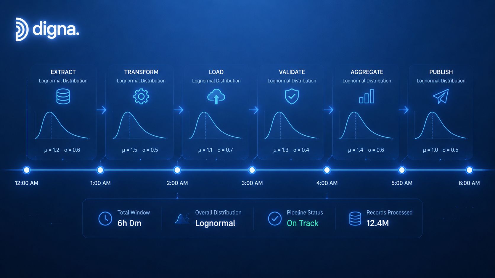
The production version should condition stage distributions on relevant features such as upstream volume or partition count. It should also compare simulated completion times with observed arrivals. A separate Python approach to data anomaly detection is useful when the same pipeline needs anomaly signals alongside timeliness forecasts.

Variance Reduction and Convergence Diagnostics

Crude Monte Carlo has a predictable weakness. The standard error of an average decreases at O(1/√N), so tightening the estimate can require disproportionately more draws. That's painful when the target is a rare SLA breach probability or a high percentile, where the estimate may move noticeably between runs.

Variance reduction improves the information obtained from each draw. Antithetic variates pair a uniform sample u with 1 - u, which can reduce variance when the response changes in opposite directions across the pair. Control variates use a correlated quantity with a known or stable expectation. In a data pipeline, expected row count versus actual row count can provide a useful control when the output depends on volume.

Stratified sampling divides the input space into latency or workload buckets, then samples deliberately from each bucket. This prevents a large, ordinary bucket from crowding out a smaller but operationally important regime.

Diagnostics that belong in the run

A running mean makes instability visible:

import numpy as np

def running_mean_and_se(values: np.ndarray) -> tuple[np.ndarray, np.ndarray]:
    values = np.asarray(values, dtype=float)
    n = np.arange(1, len(values) + 1)
    mean = np.cumsum(values) / n
    centered = values - mean
    variance = np.cumsum(centered ** 2) / np.maximum(n - 1, 1)
    se = np.sqrt(variance / n)
    return mean, se

import numpy as np

def running_mean_and_se(values: np.ndarray) -> tuple[np.ndarray, np.ndarray]:
    values = np.asarray(values, dtype=float)
    n = np.arange(1, len(values) + 1)
    mean = np.cumsum(values) / n
    centered = values - mean
    variance = np.cumsum(centered ** 2) / np.maximum(n - 1, 1)
    se = np.sqrt(variance / n)
    return mean, se

import numpy as np

def running_mean_and_se(values: np.ndarray) -> tuple[np.ndarray, np.ndarray]:
    values = np.asarray(values, dtype=float)
    n = np.arange(1, len(values) + 1)
    mean = np.cumsum(values) / n
    centered = values - mean
    variance = np.cumsum(centered ** 2) / np.maximum(n - 1, 1)
    se = np.sqrt(variance / n)
    return mean, se

For simulations organized into chains, compare within-chain and between-chain variance using an R-hat-style diagnostic:

def r_hat(chains: np.ndarray) -> float:
    """Return a lightweight split-chain R-hat estimate."""
    chains = np.asarray(chains, dtype=float)
    chain_means = chains.mean(axis=1)
    within = chains.var(axis=1, ddof=1).mean()
    between = chains.shape[1] * chain_means.var(ddof=1)
    variance = (
        (chains.shape[1] - 1) * within + between
    ) / chains.shape[1]
    return float(np.sqrt(variance / within))

def r_hat(chains: np.ndarray) -> float:
    """Return a lightweight split-chain R-hat estimate."""
    chains = np.asarray(chains, dtype=float)
    chain_means = chains.mean(axis=1)
    within = chains.var(axis=1, ddof=1).mean()
    between = chains.shape[1] * chain_means.var(ddof=1)
    variance = (
        (chains.shape[1] - 1) * within + between
    ) / chains.shape[1]
    return float(np.sqrt(variance / within))

def r_hat(chains: np.ndarray) -> float:
    """Return a lightweight split-chain R-hat estimate."""
    chains = np.asarray(chains, dtype=float)
    chain_means = chains.mean(axis=1)
    within = chains.var(axis=1, ddof=1).mean()
    between = chains.shape[1] * chain_means.var(ddof=1)
    variance = (
        (chains.shape[1] - 1) * within + between
    ) / chains.shape[1]
    return float(np.sqrt(variance / within))

A Geweke-style check compares the first and last 10% of draws with a two-sample z-score. The exact implementation should account for autocorrelation when draws aren't independent. For a practical stopping policy, require a relative standard error below 0.5% of the estimate and chain agreement within 1.01. Those thresholds should be recorded as governance settings, not applied implicitly inside a notebook.

The wider lesson appears in current Monte Carlo discussions: computational cost, critical slowing down, and the need for more efficient variants mean that “just run more simulations” is incomplete advice (Monte Carlo limitations and model-quality guidance). For a wider statistical toolkit, statistical methods for data analysis provides useful adjacent context.

Common Pitfalls That Break Production Simulations

A simulation can be perfectly reproducible and still be wrong. Most failures come from treating the random sampler as the model, while the actual defects sit in seeds, dependency structure, or data drift.

Seed mismanagement is the first signature to check. Re-seeding inside a row-level loop can repeat patterns, destroy intended independence, and make effective sample-size claims meaningless. Create one generator per independent stream, derive worker seeds deliberately, and log the seed tree with the run configuration.

Read the failure in the dashboard

Raw minute-level latency traces often contain autocorrelation. Sampling those observations as if they were independent can understate the chance of a sustained slow period. Inspect the ACF, then use a block bootstrap or model residuals with an AR(1) process before drawing synthetic sequences.

Hidden correlations create a different failure. Request size and partition count may rise together during high-volume periods, yet independent Gaussian draws produce combinations that never occur in reality. Preserve the relationship with a correlation matrix and Cholesky factorization:

import numpy as np

correlation = np.array(
    [
        [1.0, 0.7],
        [0.7, 1.0],
    ]
)

lower = np.linalg.cholesky(correlation)
independent = np.random.default_rng(42).normal(
    size=(2, 10_000)
)
correlated = lower @ independent

import numpy as np

correlation = np.array(
    [
        [1.0, 0.7],
        [0.7, 1.0],
    ]
)

lower = np.linalg.cholesky(correlation)
independent = np.random.default_rng(42).normal(
    size=(2, 10_000)
)
correlated = lower @ independent

import numpy as np

correlation = np.array(
    [
        [1.0, 0.7],
        [0.7, 1.0],
    ]
)

lower = np.linalg.cholesky(correlation)
independent = np.random.default_rng(42).normal(
    size=(2, 10_000)
)
correlated = lower @ independent

The correlation value in this example is illustrative model input, not a platform statistic. In production, estimate it from the relevant telemetry window and validate it against current behavior.

Percentiles need uncertainty too

Reporting a p99 latency from one run encourages false confidence. Bootstrap the simulated output, calculate percentile bands, and expose the interval with the point estimate. A broad band means the simulation hasn't earned a precise operational claim yet.

Other useful signatures include:

• ACF plots: Persistent correlation indicates that independent resampling is unsafe.

• Correlation heatmaps: Missing relationships reveal unrealistic joint draws.

• KS-test results: A failed fit challenges the selected parametric distribution.

• Bootstrap percentile bands: Wide bands expose unstable tail estimates.

• NaN and infinity logs: Numerical overflow often appears when probabilities become extremely small.

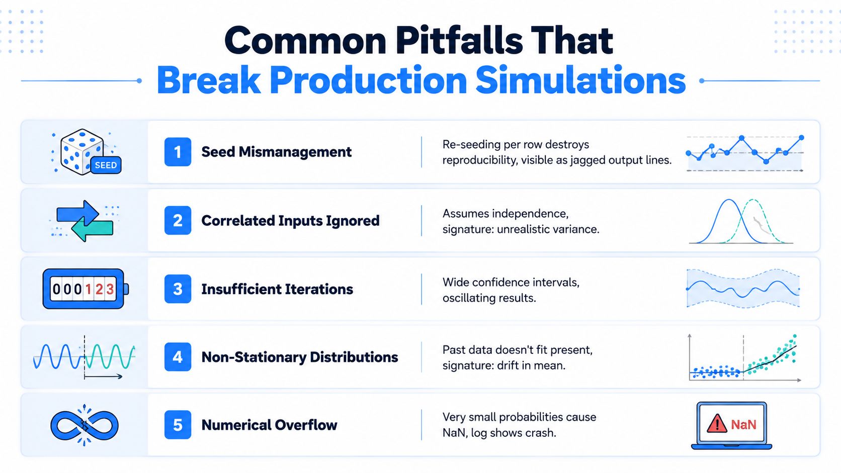
Non-stationarity deserves its own alert. A distribution fitted to an old operating regime may show a drifting mean when traffic, code, or warehouse configuration changes. Refresh inputs on a defined schedule and compare recent telemetry with the baseline before trusting the forecast.

Practical Use Cases for Data Engineers

Monte Carlo earns its compute budget when the output changes a decision. Three deployments recur in data platforms because each converts hidden uncertainty into a metric that an engineer, analyst, or incident commander can act on.

Uncertainty around business metrics

A conversion rate is an estimate, not a physical constant. For each user cohort, sample Bernoulli outcomes from a modeled conversion-rate distribution, combine the cohort results with observed or forecast traffic, and calculate a revenue outcome for each trial.

A pandas and NumPy implementation can keep the inner loop vectorized:

import numpy as np
import pandas as pd

cohorts = pd.DataFrame(
    {
        "cohort": ["new", "returning"],
        "users": [120_000, 45_000],
        "conversion_rate": [0.025, 0.061],
        "order_value": [80.0, 95.0],
    }
)

rng = np.random.default_rng(42)
trials = 20_000

rates = rng.beta(
    a=cohorts["conversion_rate"].to_numpy() * 1_000,
    b=(1 - cohorts["conversion_rate"].to_numpy()) * 1_000,
    size=(trials, len(cohorts)),
)

orders = rng.binomial(
    n=cohorts["users"].to_numpy(),
    p=rates,
)

revenue = (
    orders * cohorts["order_value"].to_numpy()
).sum(axis=1)

forecast = pd.Series(
    {
        "median": np.quantile(revenue, 0.50),
        "lower_band": np.quantile(revenue, 0.05),
        "upper_band": np.quantile(revenue, 0.95),
    }
)

import numpy as np
import pandas as pd

cohorts = pd.DataFrame(
    {
        "cohort": ["new", "returning"],
        "users": [120_000, 45_000],
        "conversion_rate": [0.025, 0.061],
        "order_value": [80.0, 95.0],
    }
)

rng = np.random.default_rng(42)
trials = 20_000

rates = rng.beta(
    a=cohorts["conversion_rate"].to_numpy() * 1_000,
    b=(1 - cohorts["conversion_rate"].to_numpy()) * 1_000,
    size=(trials, len(cohorts)),
)

orders = rng.binomial(
    n=cohorts["users"].to_numpy(),
    p=rates,
)

revenue = (
    orders * cohorts["order_value"].to_numpy()
).sum(axis=1)

forecast = pd.Series(
    {
        "median": np.quantile(revenue, 0.50),
        "lower_band": np.quantile(revenue, 0.05),
        "upper_band": np.quantile(revenue, 0.95),
    }
)

import numpy as np
import pandas as pd

cohorts = pd.DataFrame(
    {
        "cohort": ["new", "returning"],
        "users": [120_000, 45_000],
        "conversion_rate": [0.025, 0.061],
        "order_value": [80.0, 95.0],
    }
)

rng = np.random.default_rng(42)
trials = 20_000

rates = rng.beta(
    a=cohorts["conversion_rate"].to_numpy() * 1_000,
    b=(1 - cohorts["conversion_rate"].to_numpy()) * 1_000,
    size=(trials, len(cohorts)),
)

orders = rng.binomial(
    n=cohorts["users"].to_numpy(),
    p=rates,
)

revenue = (
    orders * cohorts["order_value"].to_numpy()
).sum(axis=1)

forecast = pd.Series(
    {
        "median": np.quantile(revenue, 0.50),
        "lower_band": np.quantile(revenue, 0.05),
        "upper_band": np.quantile(revenue, 0.95),
    }
)

The dashboard should show a median and uncertainty band, with the assumptions available to the people interpreting the metric. Don't present a single number as though it were measured without error.

SLA breach probability for data delivery

For a nightly pipeline, sample each stage duration conditionally on upstream volume, sum the trajectory, and publish the probability that delivery occurs after the deadline. That probability belongs beside freshness and expected arrival time, not buried in a notebook.

A timeliness system defines an expected delivery time as the learned or agreed window when a dataset, table, or partition should be ready for downstream use, then compares actual arrival with the planned schedule to alert on late or missing data (digna timeliness documentation). This complements reliability guidance that treats timeliness as a core data-quality dimension and defines latency as current time minus data creation time (timeliness as a data-quality dimension).

Synthetic anomaly data for detector benchmarking

Real anomalies are scarce and labels are often incomplete. Fit a baseline to clean data, generate synthetic observations, inject point, contextual, and collective anomalies, then replay them through the detector. The evaluation should measure precision and recall at an alert volume the on-call team can staff.

Academic work describes Monte Carlo simulation as a way to approximate ideal performance metrics when a simulated dataset can generate an unlimited number of examples, including benchmarking anomaly detectors (academic Monte Carlo benchmarking discussion). A published anomaly-detection study also ran its full evaluation loop 500 times and explicitly referred to those repetitions as 500 Monte Carlo simulations, illustrating how repetition can stabilize performance estimates (published anomaly-detection study).

These outputs should become scheduled metrics. Pair them with Great Expectations, freshness checks, volume monitors, and schema validation. Monte Carlo doesn't replace deterministic controls. It estimates how uncertain outcomes behave when those controls operate under variable conditions.

Production Checklist for Shipping a Monte Carlo Model

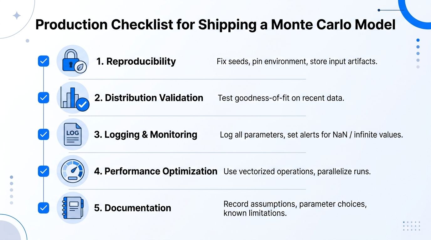
A notebook proves that code can run. A production model proves that another engineer can reproduce the result, understand the assumptions, detect degradation, and use the output during an incident.

Reproducibility and governance

Store the random seed, package environment, input snapshot, fitted distribution parameters, correlation matrix, trial configuration, and convergence diagnostics with every run. Pin dependencies and retain the exact artifacts used to create the forecast. A seed without the input data and model version isn't reproducibility, it's only a partial clue.

Version assumptions as carefully as code. Record the model owner, review date, source tables, distribution-selection rationale, and changes to filters or censoring rules. When a pipeline changes its retry policy, warehouse size, or partition strategy, treat that change as a reason to review the simulation.

Runtime controls

Use vectorized operations for the inner model and parallelize only after measuring the workload. Set resource budgets, timeouts, and failure alerts. A run that returns no result because it timed out should be a visible operational event, not a missing dashboard tile.

Alert when:

• Convergence fails: The running estimate or chain diagnostics remain unstable.

• Inputs drift: Recent telemetry no longer resembles the fitted baseline.

• Values overflow: NaN or infinite outputs appear.

• Runtime changes: Execution exceeds the agreed resource or schedule budget.

• Data is missing: The model lacks enough current observations to fit or refresh inputs.

For the surrounding pipeline architecture, document ownership and dependencies in the ETL data pipeline guidance. The simulation should compose with existing observability rather than create a parallel operating model. Its uncertainty bands belong in dashboards, and its breach probabilities belong in incident runbooks with clear actions.

A strong Monte Carlo workflow therefore has five properties: reproducible execution, validated distributions, explicit dependency structure, tested convergence, and an operational destination for every output. Without those properties, more trials only produce a more polished version of an unverified assumption.

digna provides in-environment data observability for anomalies, validation, schema changes, business metrics, and timeliness, giving teams a place to connect simulation outputs with the monitoring signals they already operate. Visit digna to see how probabilistic forecasts and data-quality controls can fit into a production reliability workflow.