Sensor Data Anomaly Detection: A Practical Guide

A vibration dashboard turns red during the afternoon shift. The operator checks the machine and finds nothing obvious. The alarm came from a temperature channel reacting to a warmer room, while a separate vibration channel has been drifting toward failure without crossing its fixed limit. By the time someone connects the signals, the detector has either cried wolf too often or stayed silent for too long.

That's the deployment reality of sensor data anomaly detection. Industrial streams are noisy, multimodal, time-dependent, and constantly changing. A detector that performs well on a clean benchmark can still fail when sensors drift, timestamps misalign, channels move together, or the plant changes operating regime. The practical question isn't only which model has the highest score. It's whether the system can identify meaningful deviations quickly enough for an operator or engineer to act.

Table of Contents

• Why Sensor Anomaly Detection Is Harder Than It Looks

  • The production constraints that matter

• Feature Engineering for Sensor Streams

  • Align time before calculating features

  • Match features to the failure pattern

  • A practical feature menu

• Choosing the Right Detection Model

  • Statistical baselines

  • Classical machine learning

  • Deep learning

• Handling Seasonality, Drift, and Correlated Channels

  • Re-anchor the baseline carefully

  • Account for coupled channels

• Evaluating Detection Performance Honestly

  • Use event-aware evaluation

• Deployment Architectures for Real-Time Monitoring

  • Match the pattern to the decision

  • Don't overlook in-database scoring

• Going Live With Confidence

  • Run the pre-launch checklist

  • Make escalation explicit

Why Sensor Anomaly Detection Is Harder Than It Looks

A turbine vibration sensor may stay nearly flat for hours after a mounting bracket loosens. The mechanical condition has changed, yet the signal can drift slowly and remain below a static threshold. A rule that alerts above one value sees normal operation. An engineer reviewing the trend, rotational context, and related channels may see an emerging fault.

That gap defines the production problem. Industrial systems combine vibration, temperature, pressure, current, control signals, images, and other modalities, each with different sampling behavior and failure modes. Missing samples create gaps, noisy readings create spikes, and correlated channels can make a legitimate operating change appear anomalous. The detector must learn normal behavior for a specific asset, operating state, and time period instead of memorizing one global range.

Practical rule: Treat “normal” as a learned operating context, not a permanent number.

Research in the field reflects the same progression. Earlier anomaly-detection methods relied heavily on statistics and signal processing. Later work expanded into machine learning and deep learning. A 2020 survey of smart anomaly detection in sensor systems describes the long history of statistical and signal-processing methods and distinguishes conventional techniques from data-driven approaches. A separate review of industrial machinery anomaly detection evaluated 84 studies spanning 2016 to 2023, illustrating the rapid growth of modern industrial research.

The production constraints that matter

A detection pipeline must address several constraints before it can produce a useful score:

• Operating-regime changes: Load, speed, ambient temperature, production recipes, and shift patterns change the expected signal.

• Sensor drift: Calibration changes and aging can shift the baseline while the machine remains healthy.

• Correlated channels: Temperature, vibration, and current may respond to the same mechanical or electrical condition.

• Uneven sampling: One channel may arrive rapidly while another reports sporadically, so naive row-by-row joins can misrepresent relationships.

• Delayed labels: Maintenance teams rarely record the exact moment an anomaly began, leaving training and evaluation windows uncertain.

• Latency and locality: A safety decision may need to happen near the machine, while deeper analysis can run in a central platform.

These conditions explain why benchmark accuracy on clean datasets often performs poorly in production. Benchmarks tend to provide orderly timestamps, stable distributions, and explicit labels. Plants provide sensor dropouts, maintenance interventions, changing workloads, and anomalies that develop over time. A model can score well while producing alerts too late, too often, or without enough context for an operator to act.

For teams responsible for the surrounding pipelines, data observability for operational reliability supplies controls for separating a machine anomaly from a late, missing, malformed, or structurally changed feed. The detector cannot reason reliably about a signal that never arrived or arrived in the wrong shape. Operational monitoring must therefore cover both the equipment and the data path that represents it.

Feature Engineering for Sensor Streams

Raw sensor values are weak model inputs without operating context. A temperature of 70 may be normal at one load and suspicious at another. A vibration reading that looks harmless alone may matter after a sustained ramp. Useful features capture local context, change over time, and relationships across channels.

Align time before calculating features

Choose an analysis cadence that matches the detector's latency budget, then resample each channel deliberately. Do not forward-fill a high-frequency vibration stream across a long outage, or interpolate through a period when the equipment was offline. Keep an imputation and missingness indicator so the detector can separate a measured value from a reconstruction.

Alignment also depends on clock quality. Clock skew between devices or gateways can create false lag relationships when one channel explains another. Check timestamp ordering, duplicates, sampling gaps, and unit consistency before joining streams. A well-designed feature built from incorrectly aligned signals is still wrong.

For multimodal equipment, preserve the original channel timestamps or quality flags where possible. A common cadence makes feature computation easier, but it can hide short gaps and make a slow channel appear more precise than it is. The right choice depends on the failure mode and the action window, not on a tidy table alone.

Match features to the failure pattern

A rolling z-score measures how far the current reading is from a recent mean relative to recent variation. A short window, such as five minutes, can expose a sudden amplitude jump. A longer window, such as 30 minutes, can reveal slower drift that a short window may absorb as normal. The familiar method computes the mean and standard deviation over a sliding window, then flags values beyond a selected threshold. One reference implementation uses a threshold of 3, which corresponds to roughly 3 out of 1,000 points under a normal distribution, as described in Ericsson's z-score anomaly detection example.

Differencing answers a separate question. First-order differences expose jumps between adjacent observations. Second-order differences expose changes in movement rate, helping identify an accelerating drift or emerging instability. Both operations can amplify noise, so smooth or aggregate highly volatile signals first. That preprocessing adds delay, which must fit the monitoring budget.

Lag features at one to ten steps give classical models a compact view of recent history. They suit processes where the next reading depends on recent values, but they increase dimensionality and become redundant when sampling is dense. Rolling percentiles describe local spread without assuming a symmetric distribution, making them useful for outliers and asymmetric operating behavior.

A practical feature menu

Cross-channel residuals often add more value than another transform of the same signal. Estimate the expected behavior of one channel from a related channel, then monitor the residual. Recheck that relationship as workloads and calibration change, because correlation can drift even while both sensors remain healthy.

For a closer examination of feature construction, consult sensor time-series anomaly detection guidance alongside asset knowledge. Feature selection matters more than feature volume. Each transform should answer a monitoring question, remain traceable in an alert, and avoid consuming more latency or compute than the operating decision allows.

Choosing the Right Detection Model

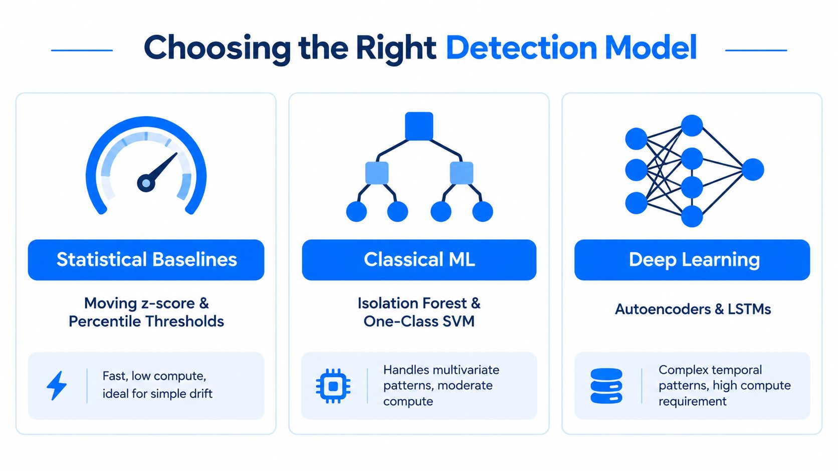
No single detector wins across every sensor regime. Statistical methods are cheap and explainable, classical machine learning handles compact multivariate spaces, and deep learning can model complicated temporal relationships. The right production design usually assigns each approach a job instead of forcing one model to process every alert.

Statistical baselines

Moving z-scores, rolling percentiles, and residual thresholds make excellent first-line detectors. They're fast, easy to inspect, and suitable for simple drift or abrupt changes. Their weakness is context. A fixed threshold breaks when the operating regime changes, and a short rolling window may treat a sustained fault as the new normal.

Adaptive baselines can remove some manual configuration. One documented implementation learns a baseline from the previous seven days of readings, updates it once per hour, and requires at least 100 readings before establishing the baseline, as described in the sensor anomaly baseline documentation. These mechanics are useful patterns, but they still need safeguards against learning from a contaminated period.

Classical machine learning

Isolation Forest and one-class SVM are useful when anomalies occupy unusual regions of a multivariate feature space. They can combine rolling statistics, lags, residuals, and operating context without requiring a large labeled failure archive. They're often easier to deploy than a sequence model, but their output can degrade when feature distributions shift or when rare faults are poorly represented.

The caution is substantial. On one industrial anomaly benchmark, Isolation Forest with or without scaling reached only 0.171 mean F1, while LOF reached 0.100 mean F1, according to the reported industrial anomaly detection results. Those results don't make the algorithms useless. They show why an unsupervised baseline must earn trust on the target equipment rather than inherit it from a textbook example.

Deep learning

LSTM autoencoders and transformer-based detectors can represent long temporal dependencies and relationships across channels. They're a better fit when the fault signature depends on a sequence rather than an isolated point, but they demand more compute, careful window design, and reliable healthy-operation data.

Applied results show both the potential and the trap. An LSTM Autoencoder combined with Isolation Forest achieved 95.7% accuracy and an F1-score of 0.93 in one sensor anomaly evaluation, as reported in this sensor anomaly identification study. A separate industrial control systems autoencoder reported 0.993 precision and 96% accuracy, but recall was only 0.673 and F1 was 0.771, documented in the industrial control systems autoencoder study. High precision can coexist with too many missed faults.

A tiered architecture is usually more effective. Let statistical rules handle obvious deviations, use classical models for multivariate residuals, and send ambiguous or temporally complex cases to a deeper model. For implementation details around Python-based anomaly workflows, Python data anomaly detection practices can sit beside your model-specific documentation.

Handling Seasonality, Drift, and Correlated Channels

A production line may run different shifts, warm through the day, and develop bearing wear while its load profile changes. A fixed threshold treats each change as a fault. The detector must separate expected movement from evidence that the process or sensor relationship has changed.

Re-anchor the baseline carefully

A rolling z-score can absorb a daily operating cycle while preserving deviations from the recent pattern. It also creates a blind spot: a fault that develops gradually across the window may become part of the baseline. Set the window from the process cycle and alerting latency, not from a convenient default.

STL decomposition separates trend, seasonal behavior, and residual variation, then scores the residual instead of the raw value. Use it when a channel has a repeatable pattern. Percentile thresholds make fewer assumptions by recalculating local bounds from recent observations, though they still require protection against contaminated training periods.

One adaptive threshold design recalculates its baseline daily from the previous seven days, uses minute-level data to estimate the 99th percentile, and adds a fluctuation term based on the interquartile range between the 25th and 75th percentiles, according to Dynatrace's auto-adaptive threshold method. The implementation illustrates a broader rule: recent behavior can define expected behavior only when abnormal periods are excluded or downweighted.

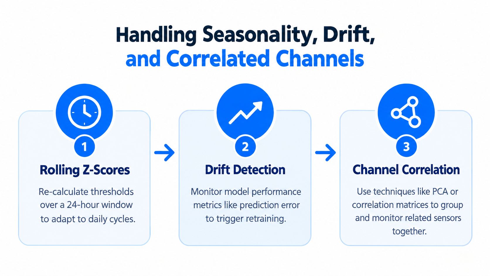
Track model drift detection for sensor baselines with model drift detection for sensor baselines. Review feature distributions, residuals, and alert outcomes separately. A baseline can look healthy even after the relationship between a sensor and its operating conditions has changed.

Account for coupled channels

Temperature, vibration, and current often move together because speed or load affects all three. Independent scoring then produces alerts for legitimate operating changes. Correlated channels should be evaluated against operating context and against one another.

Residualization is a practical first step. If RPM explains much of the vibration amplitude, regress vibration against RPM and score the residual. PCA can compress correlated channels into latent operating patterns, while correlation matrices can identify groups that belong in the same monitoring rule. Research on high-noise industrial streams also examines hybrid methods such as PCA combined with autoencoders, as discussed in this research on high-noise sensor anomaly detection.

Decision rule: Use an adaptive window when the process remains stable but its baseline moves. Retrain when the relationship between inputs and expected behavior has materially changed, or when validated incidents show systematic misses.

Keep latency in the decision. A multichannel model that misses the response budget is less useful than a simpler residual rule that runs continuously. Combine channel relationships with drift checks, then route uncertain cases for review rather than allowing the baseline to absorb them.

Evaluating Detection Performance Honestly

Accuracy is often the least useful number in an anomaly system. If faults are rare, a detector can score well by predicting normal on nearly every observation while catching nothing that matters. Even without assigning an artificial prevalence, the operational lesson is clear: evaluate the events operators care about, not just individual rows.

Precision tells you how many alerts were meaningful. Recall tells you how many labeled anomalies the detector found. Neither captures whether the system reacted early enough. Measure detection delay from anomaly onset, not merely from the end of a scoring window, because a late alert can be technically correct and operationally useless.

Use event-aware evaluation

A practical evaluation set should include:

• Precision and recall: Calculate both on labeled windows, with labels reviewed against maintenance records and operating context.

• Detection delay: Measure elapsed time from the earliest defensible anomaly onset to the first actionable alert.

• Alert volume: Track alerts per shift and per asset, not only aggregate model metrics.

• False alarm burden: Record false alarms per operator hour so the result reflects human workload.

• Missed-event review: Examine anomalies that the detector never surfaced, especially gradual drift and cross-channel failures.

A benchmark study of functional anomaly detection found that performance depends heavily on anomaly type and that simulation-based evaluation is necessary because no single detector is reliable across all patterns. That finding supports a test suite containing abrupt spikes, gradual ramps, level shifts, missing data, correlated changes, and noisy intervals, as described in the functional anomaly detection benchmark.

The literature provides a useful warning. Temporal context improved detection on an OPC UA industrial dataset by 2.27% F1, 2.33% precision, and 3.02% recall when second-order sequential memory was added, according to the industrial IoT sequential-memory study. That kind of improvement matters only if it survives a plant-specific shadow evaluation.

Run the candidate model beside existing rules in shadow mode. Keep operators blind to its alerts during the initial assessment, compare its event timing and workload with known incidents, and investigate every disagreement before promoting it.

For uncertainty analysis around rare-event scenarios, Monte Carlo simulation for operational testing can help teams explore how alert policies behave under varied signal conditions without treating a synthetic result as proof of production performance.

Deployment Architectures for Real-Time Monitoring

Architecture follows constraints. If a decision must happen close to the machine, sending every raw sample to a distant cloud adds latency and creates a dependency on network availability. If the requirement is fleet-wide trend analysis, embedding a large model in every controller creates unnecessary operational burden.

Match the pattern to the decision

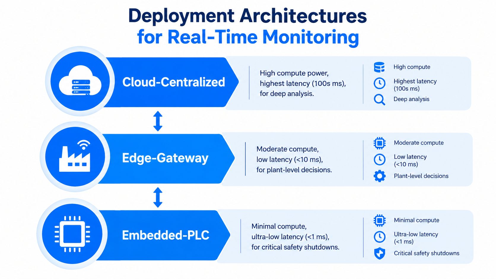
Embedded PLC or in-sensor inference suits critical local actions. A compact detector can run where the signal enters the control system, avoiding a network round trip. The trade-off is severe resource limitation, difficult model updates, and tight testing requirements. Use it for simple, safety-sensitive decisions, not automatically for every analytical workload.

Edge-gateway inference provides more room for feature engineering and multichannel models while keeping data inside the plant. A gateway can consume messages from local systems, calculate windows, and send only scores or selected features upstream. This pattern works well when privacy and resilience matter more than centralized simplicity.

Cloud or central inference offers greater compute and easier fleet-wide retraining. It fits deep analysis, cross-site comparisons, and long-horizon model development, but it depends on reliable connectivity and increases the movement of sensitive raw data.

Don't overlook in-database scoring

For fleet rollups and historical monitoring, scoring inside a time-series database such as TimescaleDB or Influx can reduce needless streaming of every point to the cloud. It also keeps feature calculations close to stored data and makes investigation easier for data engineers who already work in SQL. The limitation is that database execution may not meet hard real-time control requirements.

Cloud-edge collaboration is increasingly practical for industrial sensor networks because it separates local detection from centralized analysis. Research on cloud-edge collaborative anomaly detection describes this split as a response to latency and scalability constraints, while newer edge-oriented work focuses on real-time and resource-efficient detection.

Keep model artifacts versioned across sites. Record sensor configuration, feature definitions, calibration state, and model version with every alert. Persist enough raw context around an incident for post-hoc debugging, but define retention deliberately because raw high-frequency windows can grow quickly.

Choose based on three questions: how fast must the decision arrive, whether raw signals can leave the facility, and how much compute the local device can sustain. The answer often leads to hybrid deployment, local scoring with centralized retraining and investigation.

Going Live With Confidence

A model doesn't compensate for an untrusted alert workflow. Operators judge the system by whether alerts arrive at useful times, contain enough context, and distinguish an action-worthy event from ordinary process variation. Operational realism should decide whether a detector goes live, not architectural novelty.

Run the pre-launch checklist

Start with a shadow run beside legacy rules for two to four weeks, using the interval specified in the launch plan rather than treating it as a universal guarantee. Don't act on the new alerts yet. Compare them against maintenance records, operator notes, known interventions, and the existing alert stream.

Then tune sensitivity using observed behavior:

• Shadow run: Identify which alerts would have reached operators and whether they correspond to recognizable events.

• Threshold tuning: Balance missed events against alert burden using real operating periods, not only replayed benchmark files.

• Fallback plan: Define rollback, manual override, and safe behavior when the model, feature pipeline, gateway, or upstream data feed fails.

• Continuous monitoring: Track input drift, feature availability, score distributions, alert outcomes, and model performance after release.

Model monitoring needs an incident feedback loop. Retraining should follow verified labeled incidents and meaningful changes in operating behavior, not a calendar date chosen for convenience. If a sensor is replaced, a process changes, or a maintenance action resets the machine's behavior, record that context so the model doesn't learn the intervention as an unexplained anomaly.

Make escalation explicit

Critical anomalies should route to on-call engineers within a defined latency objective. Lower-severity events can enter a weekly review queue, where engineers examine patterns, confirm labels, and decide whether the baseline or feature set needs adjustment. Every alert should carry the asset, timestamp, contributing channels, feature values, model version, and a link to the relevant raw window.

The real success metric is operator trust. A detector earns production status when people act on its alerts without second-guessing every one.

A system that minimizes false positives on a benchmark but overwhelms a shift team has failed. A simpler detector that catches the right events, explains its score, and degrades safely can create more value than a complex model that no one can maintain. The purpose of sensor data anomaly detection is not to produce impressive metrics in isolation. It's to give the people responsible for the equipment enough timely evidence to make a better decision.

digna helps teams monitor abnormal data behavior, timeliness, validation rules, and structural changes inside their own environment, which complements sensor anomaly pipelines that depend on reliable inputs. Visit digna to see how its in-database observability approach can help you detect data gaps and unexpected movements before they undermine industrial monitoring.