Star Snowflake Schema

Your warehouse probably didn't start with a schema debate. It started with a dashboard request, a revenue report, a customer view, then a pile of new sources that all needed to land somewhere sensible. Months later, analysts are adding joins by habit, BI queries are getting slower, and nobody agrees whether the model is supposed to be simple for reporting or strict for governance.

That's where the so-called Star Snowflake Schema conversation usually appears. In practice, the phrase is misleading. Teams use it when they're no longer working with a pure star or a pure snowflake and need a practical way to talk about mixed models running in production. The core question isn't academic. It's whether your fact tables, dimensions, joins, and quality controls still support the way people query and trust the warehouse.

Most articles stop at definitions. That's not enough once a model is live, shared across teams, and changing under load. The harder problem is operational: how to choose the right pattern, where hybrid design helps, and how to monitor the breakpoints that appear when denormalized and normalized structures coexist.

Table of Contents

• The Crossroads of Data Warehouse Design

• Foundational Architectures Star and Snowflake Schemas

  • Star schema as a hub model

  • Snowflake schema as a branching model

• A Detailed Comparison of Key Differences

  • Early comparison table

  • Performance and join behavior

  • Integrity, storage, and operational maintenance

• The Rise of Hybrid Star-Snowflake Models

  • Where hybrid models appear

  • What works and what breaks

• How to Choose The Right Schema for Your Use Case

  • A practical decision lens

  • Use case starting points

• Monitoring and Observability for Your Schema

  • Schema choice is not the end of the work

  • What to monitor in mixed models

• Example Data Models and SQL Queries

  • Star schema example

  • Snowflake schema example

The Crossroads of Data Warehouse Design

A familiar pattern shows up in growing data teams. The first warehouse model is built quickly, usually around a handful of dashboards and a few well-understood sources. It works. Then the business adds regional reporting, product hierarchy changes, finance wants stricter reconciliation, and someone asks why the dashboard that used to load instantly now drags through several joins.

At that point, schema design stops being a modeling preference and becomes an operating constraint. The way you structure facts and dimensions affects query speed, BI usability, storage behavior, and how painful future changes will be. It also affects who can safely work with the model. A flattened design helps analysts move fast. A more normalized one gives engineers tighter control over dimensional consistency.

Teams rarely regret deciding deliberately. They regret inheriting a structure that grew by accident.

The phrase star snowflake schema often appears right here, at the point where a warehouse is no longer cleanly one thing or the other. That's useful shorthand in conversation, but it hides an important detail. You're not choosing a formal hybrid standard. You're deciding where to keep dimensions flat, where to normalize them, and what that means for performance, governance, and observability in production.

Foundational Architectures Star and Snowflake Schemas

The term star snowflake schema sounds like a single modeling technique. It isn't. It blends two distinct dimensional patterns that solve different problems.

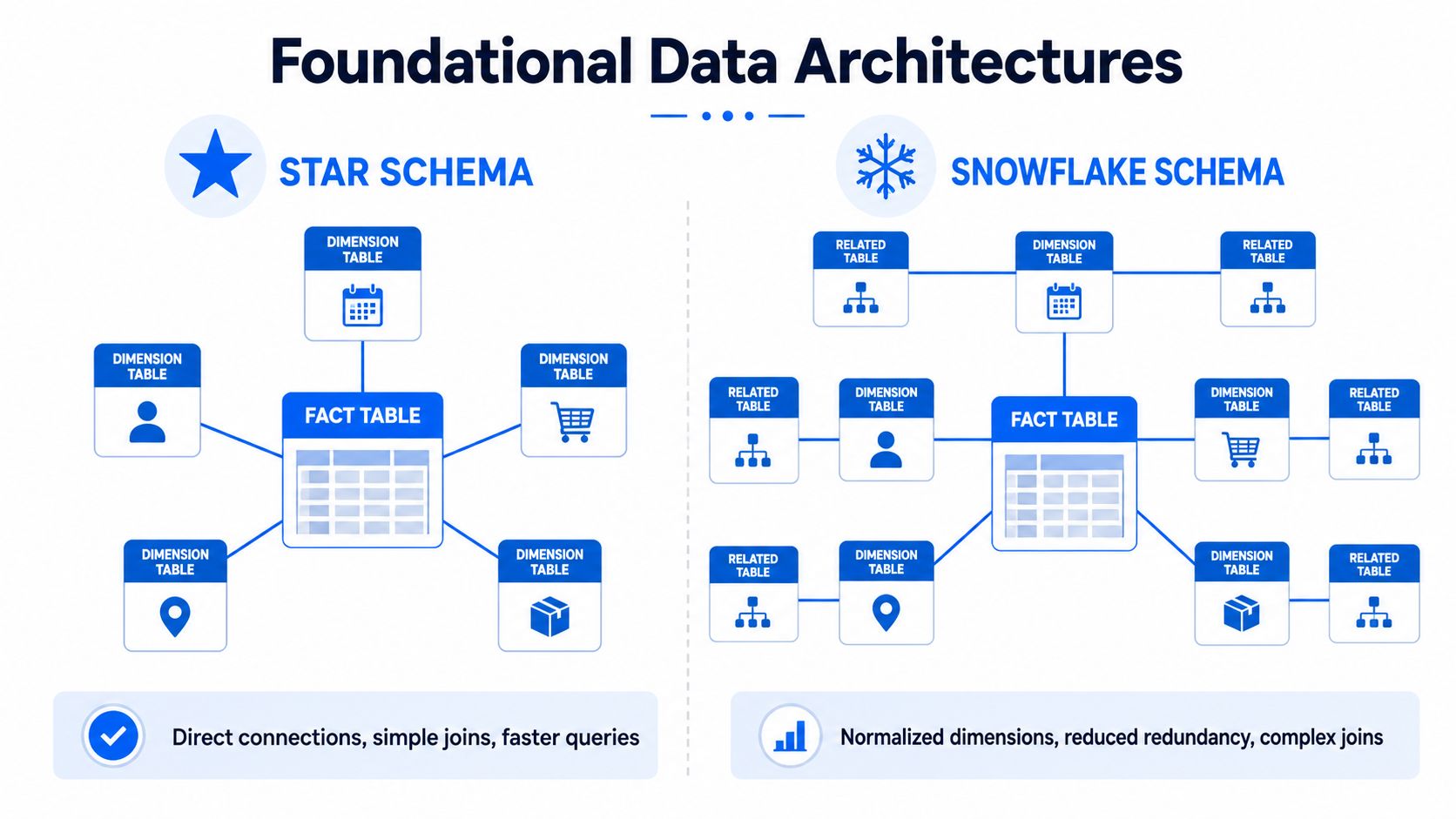
The first is the star schema. The second is the snowflake schema. According to Snowflake's explanation of star schema fundamentals, the star schema is the approach most widely used to develop data warehouses, with one or more fact tables connected to denormalized dimension tables for simpler queries and faster performance. The snowflake schema is the expanded form, where those dimensions are normalized into sub-dimension tables.

For teams designing analytical models, that difference is the whole game.

Star schema as a hub model

A star schema puts a fact table in the center and connects it directly to surrounding dimension tables. Think sales facts in the middle, then product, customer, date, and store dimensions around it. Each dimension carries the descriptive attributes analysts need for grouping and filtering.

That direct shape matters because it keeps SQL short and predictable. Analysts can join the fact table to dimensions without navigating hierarchy tables for category, region, or department. If your priority is reporting speed and model readability, this is why star schemas remain the default starting point.

A practical warehouse modeling reference like digna's warehouse data modeling guide is useful here because it frames the design choice around analytics behavior, not just textbook normalization.

Snowflake schema as a branching model

A snowflake schema starts from the same center, but dimension tables branch into related sub-dimensions. Product may split into subcategory and category tables. Geography may split into city, region, and country. The shape becomes more hierarchical, and the dimension layer reflects shared reference data more explicitly.

That normalization reduces redundancy and supports stronger consistency across dimensional attributes. If a category name changes, you update the relevant dimension row rather than repeating the change across a flatter denormalized table. The trade-off is obvious in SQL. More tables mean more joins. More joins mean more complexity in BI queries, query planning, and troubleshooting.

Practical rule: Use a star when people query constantly. Use a snowflake when dimension consistency is expensive to get wrong.

A Detailed Comparison of Key Differences

A design choice starts to matter when production traffic hits it. The difference between star and snowflake shows up in three places first: query latency, model maintenance, and the amount of monitoring required to keep dimensions trustworthy over time.

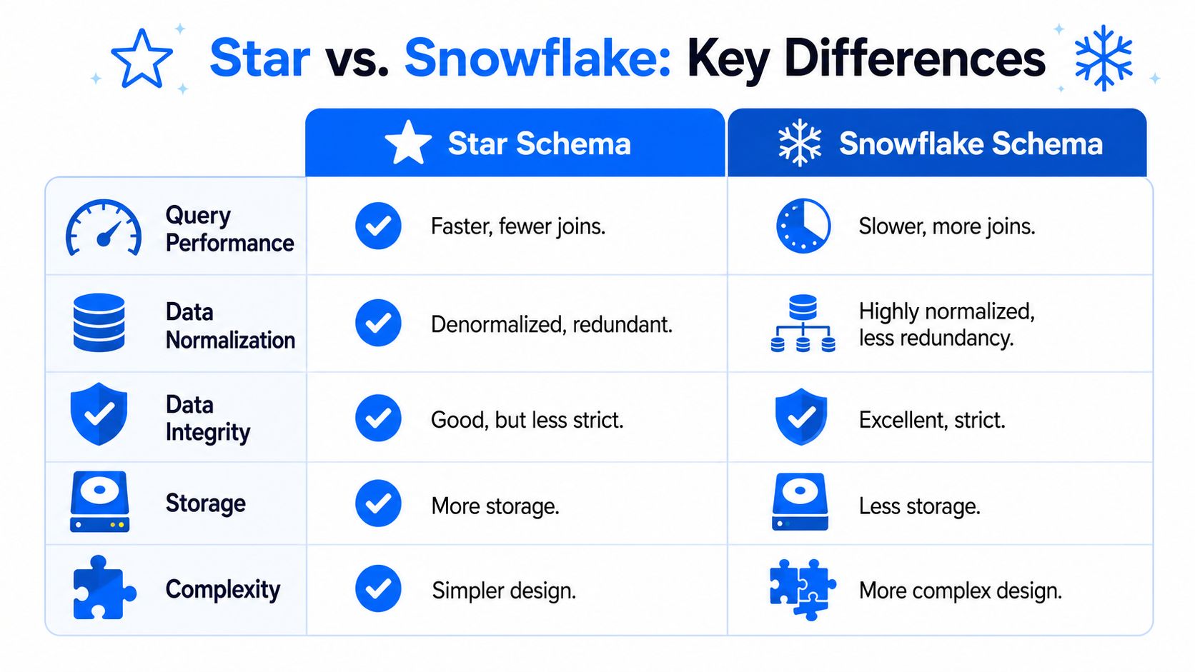
Early comparison table

Performance and join behavior

Join count is still the clearest predictor of day-to-day query behavior. In a star schema, analysts usually join the fact table to a small set of wide dimensions and stop there. In a snowflake schema, those dimensions often split into hierarchy tables, so every report that groups by category, region, or department adds more join work for the engine and more room for SQL errors.

Fivetran's comparison of star schema and one big table patterns supports the general direction of that trade-off across Redshift, Snowflake, and BigQuery. Flatter models usually read faster. That does not make snowflake a bad design. It means every normalized branch needs to justify its cost in latency, semantic complexity, and support load.

This shows up quickly in BI tooling. Semantic layers are easier to model on stars because the join graph is smaller and more stable. Query plans are also easier to reason about during incident response. When a dashboard slows down after a schema change, a flat dimension model gives engineers fewer places to inspect.

Integrity, storage, and operational maintenance

Snowflake schemas earn their place when dimensional consistency has a real operational cost. Product taxonomy, legal entity structures, regulated customer classifications, and geography hierarchies often change under tighter governance than the facts that reference them. Normalizing those structures reduces duplicate attributes and lowers the chance that two reports use different versions of the same reference value.

Storage efficiency is a secondary benefit now that warehouse compute usually costs more attention than raw disk. The larger issue is change management. A star schema pushes complexity into ETL or ELT pipelines that flatten dimensions before analysts query them. A snowflake schema keeps the reference model cleaner, but it shifts more complexity into joins, semantic definitions, and dependency tracking.

That trade-off affects different teams in different ways:

• Analysts write shorter SQL against stars and spend less time tracing hierarchy logic across multiple tables.

• Data engineers spend less time exposing curated marts on simple stars, but more time managing duplicated attributes and backfills when dimension values drift.

• BI developers and analytics engineers do more semantic modeling work on snowflakes because every additional branch needs tested join logic, clear naming, and guardrails against fan-out errors.

• Platform teams need stronger observability on snowflakes. Broken hierarchy links, orphaned keys, and delayed dimension loads can degrade report correctness without causing a hard pipeline failure.

In production, that last point matters more than many design guides admit. A star schema usually fails in visible ways, such as stale denormalized attributes or slower rebuilds. A snowflake schema can fail subtly. One missing row in a sub-dimension can change aggregates, drop categories from dashboards, or produce inconsistent drill paths across tools. That is why schema choice should include an operational question, not just a modeling one: which failure mode is easier for your team to detect, explain, and fix?

The Rise of Hybrid Star-Snowflake Models

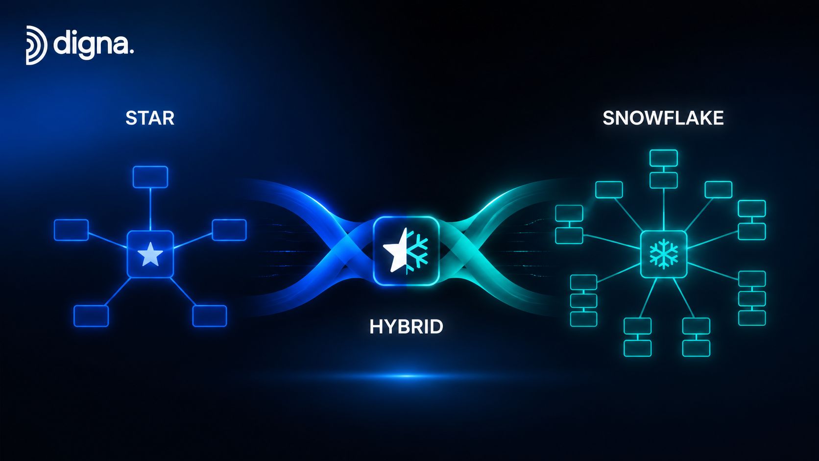
Very few production warehouses stay pure for long. Product dimensions stay flat because analysts hit them every day. Geography gets normalized because regional hierarchies change. Customer attributes split because governance rules require tighter control over some fields but not others. This describes what is often termed a star snowflake schema.

It isn't a third canonical architecture. It's a practical mixed model.

Where hybrid models appear

Hybrid patterns usually emerge in one of three ways.

• A mostly star warehouse with one snowflaked dimension. This is common with geography, product taxonomy, or organizational hierarchy.

• A governed core with flattened marts. The warehouse keeps normalized reference dimensions, then downstream marts expose denormalized views for BI consumption.

• A model that evolved over time. New dimensions were added under different constraints, so some remained flat while others were normalized.

That mixed approach is often reasonable. According to Big Data Boutique's comparison, star schemas remain the optimal starting point for 90% of analytics use cases, with snowflake patterns reserved for large dimensions or strict governance requirements.

What works and what breaks

What works is selective normalization. A team can keep high-traffic dimensions flat for dashboard performance and snowflake the few dimensions where redundancy or governance cost is real. That can be a disciplined design.

What doesn't work is accidental inconsistency. One dimension follows conformed naming. Another stores duplicate attributes in two places. Analysts don't know whether category should come from the flat product table or the normalized category table. SQL starts returning technically valid but logically inconsistent answers.

A hybrid model also increases operational burden:

Hybrid models fail when teams mix patterns without naming, ownership, and validation discipline.

How to Choose The Right Schema for Your Use Case

A schema decision usually gets forced by a production problem, not by theory. A BI team is fielding complaints about slow dashboards. A governance lead is finding conflicting product hierarchies in finance and sales reports. A platform team is spending too much time repairing dimension updates after source changes. The right choice starts with the failure mode you need to reduce.

A practical decision lens

Start with the query path. If analysts, BI developers, or downstream tools hit warehouse tables directly, star is usually the safer default because it keeps joins predictable and makes semantic errors easier to spot. If a semantic layer hides model complexity, you have more room to normalize, but the maintenance cost does not disappear. Data engineers still own the joins, key management, and hierarchy logic underneath.

The next question is change frequency. Snowflaking pays off when dimension structures change often enough that repeated attribute updates become a real operational cost. Product taxonomy, legal entity rollups, regional mappings, and chart of accounts are common examples. In those cases, normalization is less about elegance and more about controlling update paths, reducing duplicate business logic, and lowering the odds that one report uses stale reference data.

Performance still matters, but the trade-off is broader than join count. Star schemas usually make ad hoc analysis faster and easier to tune. Snowflake schemas can improve consistency in shared dimensions, but they also create more dependencies, more lineage to track, and more ways for upstream changes to break downstream queries.

Use these questions to make the decision concrete:

1. Who owns the last mile of querying? Direct SQL users usually do better with flatter dimensions.

2. Which dimensions change structurally, not just by row count? Frequent hierarchy changes often justify normalization.

3. Where does bad data create the highest cost? If duplicate or conflicting reference values create audit, finance, or compliance issues, control may matter more than speed.

4. How many downstream models reuse the same dimension logic? Shared logic pushes the design toward stronger central control.

5. Can the team monitor the model well enough to support extra complexity? A snowflaked or hybrid design needs tighter lineage, freshness checks, and key integrity monitoring. Teams that already invest in data observability practices can handle that complexity more safely.

Use case starting points

Some defaults hold up well in practice.

• Retail sales analytics: Start with star. Product, store, customer, and date dimensions are filtered constantly, and dashboard responsiveness usually matters more than reducing a modest amount of dimensional redundancy.

• Financial reporting with controlled hierarchies: Start with selective snowflaking or a governed hybrid. Account and entity structures change under formal controls, and inconsistent rollups create reporting risk quickly.

• User behavior and product analytics: Keep it flat unless a dimension is both large and heavily reused. These teams change definitions fast, and every extra join slows analysis and raises the odds of inconsistent SQL.

• Healthcare and regulated operations: Expect a hybrid. Reporting users still need usable marts, but provider, location, code set, and organizational reference data often need tighter control and clearer ownership.

A short decision check catches many bad implementations:

• Ask the BI team which dimensions drive most filters, drill paths, and dashboard latency.

• Ask governance owners which attributes must come from one controlled table.

• Ask analysts where join logic already causes inconsistent answers.

• Ask platform engineers which dimensions fail most often during source schema changes or late-arriving updates.

If those answers are vague, the design is not ready. The schema should reflect how the warehouse is operated, monitored, and debugged in production, not just how it looks on a whiteboard.

Monitoring and Observability for Your Schema

Schema design isn't a one-time choice. It's an operating surface that keeps changing under ingestion updates, model revisions, source application releases, and new downstream consumers. The model that was correct last quarter can become fragile without anyone formally redesigning it.

That's especially true for a star snowflake schema in the practical sense of a mixed production model.

Schema choice is not the end of the work

Teams often monitor pipeline success and warehouse cost, but they don't monitor the model itself closely enough. That gap shows up as schema drift, silent distribution drift in fact tables, late-arriving dimensions, orphaned foreign keys, or business logic that passes structurally while failing analytically.

The problem gets sharper in hybrid environments. ThoughtSpot's discussion of schema complexity notes that 40% of analytics teams now use hybrid models to balance query speed and storage, while mainstream guidance still leaves a gap around validating record-level business logic across these inconsistent structures.

A general observability program for these models should watch four things:

• Structural changes: Added columns, removed columns, and data type changes in fact or dimension tables.

• Relational health: Broken foreign keys, missing dimension rows, and mismatched hierarchy mappings.

• Behavioral drift: Unexpected shifts in volume, value distributions, or null patterns even when the schema hasn't changed.

• Delivery timing: Late loads that don't break SQL but do break trust in reports.

What to monitor in mixed models

One practical option is digna's data observability approach, particularly when a team needs in-database monitoring inside a private cloud or on-prem environment. The platform documentation states that metric computation, baselines, and trend analysis run inside the customer database with zero data movement, and its Schema Tracker flags structural changes such as added or removed columns and data type changes in real time. Its anomaly detection learns normal behavior for timing and seasonal patterns and can detect deviations in record volumes, distributions, compound business key issues, and foreign key orphaned records. Timeliness monitoring also tracks expected delivery patterns so delays are caught before they propagate into reports.

That matters because star and snowflake models fail differently. In a star design, denormalized dimensions tend to hide duplication and stale descriptive attributes. In a snowflake design, the risk shifts toward broken join chains, missed hierarchy updates, and latent performance regressions. In a hybrid model, you get both classes of failure.

Don't just monitor whether tables loaded. Monitor whether the model still means what your users think it means.

Example Data Models and SQL Queries

The design difference becomes obvious once you write SQL against both patterns. Below is the same sales use case modeled two ways: total sales by product category and customer region.

Star schema example

A star model keeps category and region directly in the dimensions most analysts already use.

CREATE TABLE fact_sales (
  sale_id BIGINT,
  date_id INT,
  product_id INT,
  customer_id INT,
  quantity INT,
  revenue NUMERIC(18,2)
);

CREATE TABLE dim_product (
  product_id INT,
  product_name VARCHAR(255),
  category_name VARCHAR(255)
);

CREATE TABLE dim_customer (
  customer_id INT,
  customer_name VARCHAR(255),
  region_name VARCHAR(255)
);

CREATE TABLE dim_date (
  date_id INT,
  calendar_date DATE,
  month_name VARCHAR(20),
  year_num INT
);

CREATE TABLE fact_sales (
  sale_id BIGINT,
  date_id INT,
  product_id INT,
  customer_id INT,
  quantity INT,
  revenue NUMERIC(18,2)
);

CREATE TABLE dim_product (
  product_id INT,
  product_name VARCHAR(255),
  category_name VARCHAR(255)
);

CREATE TABLE dim_customer (
  customer_id INT,
  customer_name VARCHAR(255),
  region_name VARCHAR(255)
);

CREATE TABLE dim_date (
  date_id INT,
  calendar_date DATE,
  month_name VARCHAR(20),
  year_num INT
);

CREATE TABLE fact_sales (
  sale_id BIGINT,
  date_id INT,
  product_id INT,
  customer_id INT,
  quantity INT,
  revenue NUMERIC(18,2)
);

CREATE TABLE dim_product (
  product_id INT,
  product_name VARCHAR(255),
  category_name VARCHAR(255)
);

CREATE TABLE dim_customer (
  customer_id INT,
  customer_name VARCHAR(255),
  region_name VARCHAR(255)
);

CREATE TABLE dim_date (
  date_id INT,
  calendar_date DATE,
  month_name VARCHAR(20),
  year_num INT
);

Query:

SELECT
  p.category_name,
  c.region_name,
  SUM(f.revenue) AS total_revenue
FROM fact_sales f
JOIN dim_product p
  ON f.product_id = p.product_id
JOIN dim_customer c
  ON f.customer_id = c.customer_id
GROUP BY
  p.category_name,
  c.region_name
ORDER BY
  total_revenue DESC;

SELECT
  p.category_name,
  c.region_name,
  SUM(f.revenue) AS total_revenue
FROM fact_sales f
JOIN dim_product p
  ON f.product_id = p.product_id
JOIN dim_customer c
  ON f.customer_id = c.customer_id
GROUP BY
  p.category_name,
  c.region_name
ORDER BY
  total_revenue DESC;

SELECT
  p.category_name,
  c.region_name,
  SUM(f.revenue) AS total_revenue
FROM fact_sales f
JOIN dim_product p
  ON f.product_id = p.product_id
JOIN dim_customer c
  ON f.customer_id = c.customer_id
GROUP BY
  p.category_name,
  c.region_name
ORDER BY
  total_revenue DESC;

That query is short, readable, and hard to misuse. For most BI workloads, that's the point.

Snowflake schema example

A snowflake model moves category and region into normalized hierarchy tables.

CREATE TABLE fact_sales (
  sale_id BIGINT,
  date_id INT,
  product_id INT,
  customer_id INT,
  quantity INT,
  revenue NUMERIC(18,2)
);

CREATE TABLE dim_product (
  product_id INT,
  product_name VARCHAR(255),
  category_id INT
);

CREATE TABLE dim_category (
  category_id INT,
  category_name VARCHAR(255)
);

CREATE TABLE dim_customer (
  customer_id INT,
  customer_name VARCHAR(255),
  region_id INT
);

CREATE TABLE dim_region (
  region_id INT,
  region_name VARCHAR(255)
);

CREATE TABLE dim_date (
  date_id INT,
  calendar_date DATE,
  month_name VARCHAR(20),
  year_num INT
);

CREATE TABLE fact_sales (
  sale_id BIGINT,
  date_id INT,
  product_id INT,
  customer_id INT,
  quantity INT,
  revenue NUMERIC(18,2)
);

CREATE TABLE dim_product (
  product_id INT,
  product_name VARCHAR(255),
  category_id INT
);

CREATE TABLE dim_category (
  category_id INT,
  category_name VARCHAR(255)
);

CREATE TABLE dim_customer (
  customer_id INT,
  customer_name VARCHAR(255),
  region_id INT
);

CREATE TABLE dim_region (
  region_id INT,
  region_name VARCHAR(255)
);

CREATE TABLE dim_date (
  date_id INT,
  calendar_date DATE,
  month_name VARCHAR(20),
  year_num INT
);

CREATE TABLE fact_sales (
  sale_id BIGINT,
  date_id INT,
  product_id INT,
  customer_id INT,
  quantity INT,
  revenue NUMERIC(18,2)
);

CREATE TABLE dim_product (
  product_id INT,
  product_name VARCHAR(255),
  category_id INT
);

CREATE TABLE dim_category (
  category_id INT,
  category_name VARCHAR(255)
);

CREATE TABLE dim_customer (
  customer_id INT,
  customer_name VARCHAR(255),
  region_id INT
);

CREATE TABLE dim_region (
  region_id INT,
  region_name VARCHAR(255)
);

CREATE TABLE dim_date (
  date_id INT,
  calendar_date DATE,
  month_name VARCHAR(20),
  year_num INT
);

Query:

SELECT
  cat.category_name,
  r.region_name,
  SUM(f.revenue) AS total_revenue
FROM fact_sales f
JOIN dim_product p
  ON f.product_id = p.product_id
JOIN dim_category cat
  ON p.category_id = cat.category_id
JOIN dim_customer c
  ON f.customer_id = c.customer_id
JOIN dim_region r
  ON c.region_id = r.region_id
GROUP BY
  cat.category_name,
  r.region_name
ORDER BY
  total_revenue DESC;

SELECT
  cat.category_name,
  r.region_name,
  SUM(f.revenue) AS total_revenue
FROM fact_sales f
JOIN dim_product p
  ON f.product_id = p.product_id
JOIN dim_category cat
  ON p.category_id = cat.category_id
JOIN dim_customer c
  ON f.customer_id = c.customer_id
JOIN dim_region r
  ON c.region_id = r.region_id
GROUP BY
  cat.category_name,
  r.region_name
ORDER BY
  total_revenue DESC;

SELECT
  cat.category_name,
  r.region_name,
  SUM(f.revenue) AS total_revenue
FROM fact_sales f
JOIN dim_product p
  ON f.product_id = p.product_id
JOIN dim_category cat
  ON p.category_id = cat.category_id
JOIN dim_customer c
  ON f.customer_id = c.customer_id
JOIN dim_region r
  ON c.region_id = r.region_id
GROUP BY
  cat.category_name,
  r.region_name
ORDER BY
  total_revenue DESC;

The extra joins aren't catastrophic. They're just cumulative. One or two are manageable. A deeper hierarchy across several dimensions becomes harder to maintain, explain, and optimize.

In practice, that's why many teams land on a selective hybrid. They keep the dimensions that analysts touch constantly in a star-like form and normalize the dimensions that need stronger control.

If your warehouse is already mixing flat and normalized dimensions, the hard part isn't naming the pattern. It's keeping the model reliable as structures and data behavior change. digna is one option for teams that need schema tracking, anomaly detection, timeliness monitoring, and record-level validation inside their own database environment without moving production data outside their control.