Model Drift Detection: A Practical Guide for 2026

You usually don't notice model drift when it starts. The dashboards stay green, the model keeps scoring, and the first signal comes from a business user who says approvals, approvals, or recommendations feel “off” compared with last month. By the time someone opens a ticket, the model has often been running on stale assumptions for days, sometimes longer, and the team is already debugging the wrong layer.

That's why model drift detection has to start as a data observability problem. The model is only one part of the system. Inputs shift, schemas break, labels arrive late, confidence changes imperceptibly, and the output distribution starts to wobble before any obvious accuracy drop shows up.

Table of Contents

• When a Model Quietly Stops Working

• The Four Drift Types You Actually Need to Distinguish

  • Start with data drift

  • Separate concept drift from input drift

  • Treat label drift and feature drift differently

• Choosing the Right Metric for Each Signal

• Building the Detection Pipeline End to End

  • Capture the signals that make drift visible

  • Compute profiles close to the data

  • Run drift detection on slices, not just globally

  • Alert on action, not noise

• Why Performance Metrics Catch Drift Too Late

• Baselines, Thresholds, and Alert Routing That Actually Work

• Root Cause Analysis and Where Observability Fits

When a Model Quietly Stops Working

A fraud model can look healthy for weeks while the business bleeds. The dashboards show normal traffic, the model still returns scores, and no one sees anything alarming until a payments lead asks why a familiar customer segment is getting declined more often than expected. That's the painful part of drift. It doesn't always arrive as a crash, it often arrives as a change in behavior that humans notice before monitoring does.

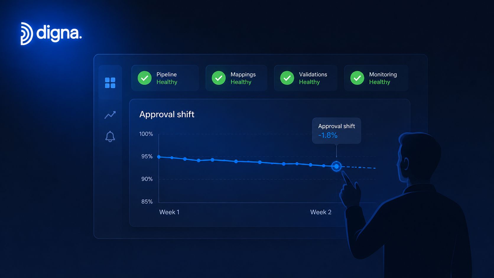
A good drift program catches that shift before the complaint lands in Slack. The practical job is not just to watch accuracy, it's to watch the system that feeds the model, the predictions it emits, and the timing of the labels that eventually confirm whether it was right. That's the difference between a model monitor and a real data observability layer for ML.

Practical rule: if a stakeholder notices the drift before the platform does, the platform is monitoring the wrong thing.

The useful mental model is simple. Input drift shows up when feature distributions change. Output drift shows up when score distributions or confidence move. Schema drift shows up when columns change shape, disappear, or arrive late. Label lag hides the truth until long after the prediction went live. You need all four in view because any one of them can break the model's usefulness without a dramatic drop in the usual KPIs.

That's why enterprise teams end up treating model drift detection as part of the broader pipeline, not as a model-only add-on. Once you frame it that way, the fix becomes clearer. You don't just retrain faster, you detect upstream change faster, localize it faster, and route it to the right owner faster.

The Four Drift Types You Actually Need to Distinguish

Data drift, concept drift, label drift, and feature drift are related, but they don't call for the same response. In production, mixing them up wastes time. A team may spend half a day retraining a model that needs a schema fix, or they may keep tuning features when the underlying relationship has changed.

Start with data drift

Data drift is the easiest to spot and the easiest to overreact to. It means the input distribution changed, while the business task may still be the same. A credit risk model might see a shift in applicant income bands after a new product launch, or a churn model might ingest more mobile users after a channel mix change. The model isn't necessarily wrong yet, but its world has changed enough that its assumptions may no longer hold.

Separate concept drift from input drift

Concept drift is the harder one. The relationship between inputs and the target changes, even if the inputs still look familiar. A fraud model may keep seeing the same transaction patterns, but criminals change tactics so the old signals stop predicting fraud as well as they used to. That's not a feature issue. It's a problem with the learned mapping itself.

Treat label drift and feature drift differently

Label drift means the class balance changes. In a credit workflow, the mix of approved versus rejected cases can move, and that alone can distort metrics and thresholds. Feature drift is narrower, it's about a specific input changing, such as a new categorical value, a widening numeric range, or a missing field that wasn't missing before. Feature drift often comes from upstream data problems rather than model behavior, which is why the response is usually pipeline repair, not retraining.

A useful checkpoint is to ask two questions. Did the inputs change, or did the relationship change? And is the issue in the model, or in the data path feeding it?

The distinction matters because a schema break, a null spike, or a delayed table can look like drift in a dashboard even when the model logic is fine. For a concrete implementation path, the digna data drift detection guide is useful because it centers the operational signals around the data layer rather than assuming labels will save you.

Choosing the Right Metric for Each Signal

The best metric depends on what you're watching and how fast you need to act. In regulated environments, teams usually want a transparent statistic tied to a baseline. In faster-moving environments, they often need a metric that can run continuously across multiple slices without becoming noisy.

The oldest and still most practical foundation is formal hypothesis testing. Kolmogorov–Smirnov (KS) works well for continuous variables because it compares the shape of live and reference distributions without assuming normality. Chi-square is the natural fit for categorical inputs, where you care about whether the category mix changed enough to matter. Population Stability Index (PSI) is widely used as a threshold-based stability check, and a PSI above 0.25 is commonly treated as a strong warning signal Statsig on drift methods and PSI.

For distributions that are more complex, Jensen-Shannon divergence is a sensible option, especially for categorical outputs, embeddings, or prediction-space monitoring. It's useful when you care about how two probability distributions differ, not just whether a single feature crossed a line. The key is not to pick one metric and pretend it covers every signal.

A single metric rarely covers all failure modes. The right stack uses one statistic for the feature, another for the output, and a third for the slice where the business cares most.

The practical default is to run multiple statistics in parallel on both short and long windows. Short windows catch incidents quickly. Long windows catch slow decay that doesn't trip a single-day check. If you're deciding where to start, the how to describe distribution of data guide is a good reference point for thinking about which shape of distribution you're comparing.

Building the Detection Pipeline End to End

A production drift pipeline has five jobs, and each job answers a different question. First, capture the right signals. Then compute profiles. Then compare live behavior to a reference. Then alert the right team. Finally, force a response, whether that's investigation, recalibration, retraining, or a pipeline fix.

Capture the signals that make drift visible

The minimum capture set is straightforward, but teams still miss pieces of it. You need model inputs, outputs, prediction confidence, timestamps, and ground-truth labels when they eventually arrive. If you're monitoring an LLM workflow, capture prompts, responses, token counts, latency, and guardrail activations as well. Those extra signals matter because silent failures in generative systems often show up in behavior, not in a single accuracy number.

Compute profiles close to the data

The profile layer should compare production behavior to a reference profile, not just to a one-off snapshot. In practice, that means storing baseline statistics and computing live metrics on the same table families over time. You want this computation close to the data, ideally in the warehouse or lake, because moving large datasets into a separate analytics store creates lag, copy overhead, and more places for the monitoring path to fail.

Run drift detection on slices, not just globally

Global averages hide localized failures. A model can look stable overall while one geography, product line, or channel is degrading. That's why production monitoring needs segmentation. Short windows help with incidents, long windows help with slow decay, and both should be broken out by the slices that matter to the business.

Alert on action, not noise

Alerting should be tied to a response path. A weak feature shift may belong in a dashboard. A sudden distribution break may deserve a page. A validation failure may need to go to the data engineering owner, not the ML team. The response only works when the signal lands with the person who can fix the underlying issue.

For teams building this in a platform setting, a tool like digna fits naturally when the goal is to compute baselines inside the warehouse and pair them with anomaly, timeliness, schema, and validation checks. That keeps the data resident where it already lives and gives operators one place to inspect trend, freshness, and structural change.

Why Performance Metrics Catch Drift Too Late

Teams love accuracy charts because they're familiar. The problem is that accuracy, precision, recall, F1, MAE, RMSE, and AUC-ROC are usually downstream signals, not early warnings. If the labels arrive late or sparsely, the metric tells you the model is off only after the business impact has already started.

That delay is the core operational problem. A model can continue serving predictions while the ground truth is still missing. By the time a meaningful drop in performance is visible, the model may have been wrong for long enough to affect approvals, fraud catches, recommendations, or service routing.

Operational truth: performance metrics are confirmation tools, not always detection tools.

This is why proxy signals matter. Input distribution shifts can show you that the incoming population changed. Prediction distribution shifts can show you that the model's confidence moved even before labels land. Shadow deployments can expose side-by-side behavior. Confidence calibration can show that the model still sounds certain while becoming less reliable. Those proxies do not prove the model has failed, but they are often the first evidence that something changed.

The most useful way to explain this internally is to treat drift flags as leads, not proof of failure. That framing keeps the team from overreacting to every blip, while still giving them permission to investigate before the backlog becomes a business incident. In high-stakes workflows, especially where labels are delayed or incomplete, that's the only stance that works reliably.

Baselines, Thresholds, and Alert Routing That Actually Work

A drift program becomes trusted when its baselines match reality. A frozen training-period baseline is good for launch, but it often ages poorly in live systems. A rolling production baseline is better for workflows that naturally evolve. Shadow-mode baselines can help when a model is being evaluated beside an incumbent, because they reflect current traffic without contaminating the main decision path.

The mistake many teams make is assuming one static threshold can cover everything. It can't. Sudden changes deserve faster escalation than slow creep. A feature that changes shape gradually may justify a warning and an investigation queue, while a sudden KS jump on a sensitive field may need immediate triage. The threshold should reflect both the metric and the operational context.

A layered routing model works better than a shared inbox. Route schema issues to the data engineering owner. Route confidence or output shifts to the ML platform or modeling team. Route freshness and missing loads to the pipeline owner. That split matters because the first responder shouldn't have to guess where the break happened.

If the alert doesn't name an owner, it isn't an alert. It's just noise with better formatting.

The fastest way to reduce alert fatigue is to make the alert informative enough to shorten the first investigation. Include the affected slice, the comparison window, the metric that moved, and the reference baseline. Then let the responder decide whether the fix is retraining, recalibration, feature repair, or a handoff to data engineering.

Root Cause Analysis and Where Observability Fits

A good drift alert should lead to a fix, not a debate. Consider a payment feature that suddenly triggers a KS spike. The model team may suspect concept drift first, but the actual cause can be a schema change upstream, such as a field being retyped or a nullable column suddenly arriving with unexpected values. In that case, the right fix is pipeline repair, not retraining.

A different case looks softer. A PSI trend rises slowly after a product launch, and the team sees worse model behavior on a subset of traffic. That often points to a customer mix shift, not a broken model. The model may still be valid, but its reference population is no longer representative. That's where historical context matters, because a trend without history is just a point in time.

The third pattern is calibration drift. The model still returns scores, but delayed labels eventually show that confidence no longer tracks reality as well as it used to. That's a reminder that monitoring has to handle late labels gracefully. Proxy signals get you early warning, while the eventual labels confirm whether the concern was real.

A data observability platform should make this investigation faster by exposing schema tracking for added or removed columns, timeliness monitoring for missing or late arrivals, anomaly detection for unexpected shifts, and historical trend views for context. That's where digna fits in practice, because it computes baselines and runs anomaly, timeliness, schema, and validation checks inside the customer's database. The benefit is not just privacy, it's also a cleaner triage path, since engineers can inspect the signal without moving sensitive data into another system.

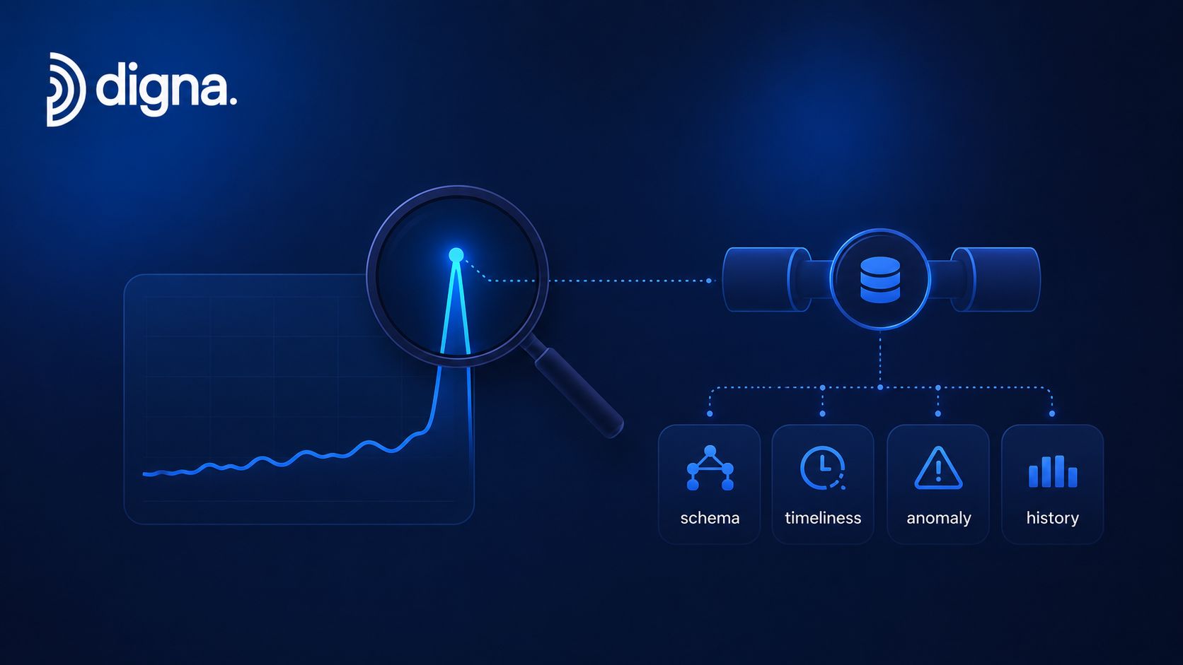
If your team is still waiting for labels before investigating drift, the monitoring loop is already too slow. Visit digna to see how warehouse-native baselines, anomaly checks, timeliness monitoring, schema tracking, and validation can give your ML systems a cleaner drift signal and a faster path from alert to root cause.