Monitor Expected Delivery Time for Data Pipelines
|
6
min read

Your executive dashboard says yesterday's pipeline is healthy, but the numbers are stale. A nightly load slipped, the table landed hours late, and nobody noticed until the meeting started. That's the kind of miss that turns expected delivery time from a logistics phrase into a daily operating signal for data teams.
In practice, the problem is rarely a single broken job. It's the gap between when a dataset should arrive, when it lands, and whether downstream users can trust the result before they make a decision. The strongest teams treat that gap as a measurable system property, not a vague annoyance.
Table of Contents
Statistical and Machine Learning Methods for Learning Arrival Windows
Handling Seasonality and Business Schedules in Arrival Estimates
In-Database Implementation Tips with digna Timeliness and Analytics
Why Expected Delivery Time Matters for Data Teams
A Monday morning dashboard that shows Friday's numbers is usually not a reporting bug, it's a timeliness failure. The load arrived late, the warehouse accepted it, and the business found out only after someone asked why the KPIs looked frozen. That's exactly why expected delivery time belongs in the same conversation as freshness, completeness, and correctness.
In the data context, expected delivery time is the learned or agreed window when a dataset, table, or partition should be populated and ready for downstream use. Unlike shipping dates, which are often framed as a single destination moment, data arrival is shaped by orchestration schedules, upstream source behavior, cutoff times, and business calendars. A rigid cron check can say “job ran,” while the actual question is whether the data arrived when consumers needed it.
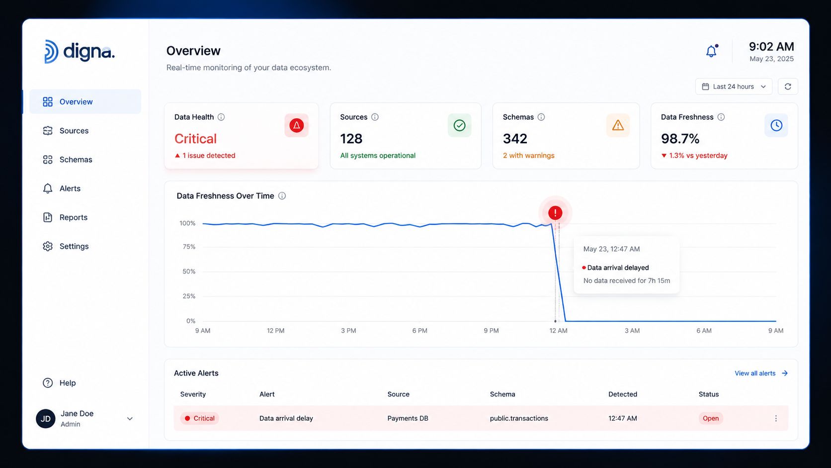
Practical rule: if a table feeds a meeting, a model, or a regulatory extract, timeliness is a product requirement, not a backend detail.
Static cron-based assumptions fail because they encode hope, not behavior. Upstream systems drift, batch windows move, and one late partition can poison several downstream jobs before anyone opens a log. Once a team starts measuring expected delivery time explicitly, stale reports stop being a surprise and start being a tracked reliability issue.
Statistical and Machine Learning Methods for Learning Arrival Windows
Teams that only store a scheduled run time end up with brittle alerts. The better model is a learned arrival window, where historical behavior defines what “on time” usually means for each table, partition, or file group. That shift turns a single timestamp into a distribution, which is much closer to how pipelines behave.
Start with statistical baselines
The simplest baseline is still useful. Rolling averages give you a moving center of gravity for arrival times, while percentile windows, such as P50, P80, and P95, show how wide the normal spread really is. Tracking coefficient of variation helps separate a stable feed from one that swings wildly from run to run, which matters more than raw mean time in many pipelines.
A useful internal pattern is to compute line-level metrics for actual lead time, promised lead time, and the deviation between them. That matches the observability guidance in digna's statistical pattern recognition overview, where the point is not to chase a single expected timestamp but to detect repeatable structure in timing behavior.
Add machine learning when behavior stops being uniform
ML becomes valuable when the baseline itself changes with source system load, regional cutovers, or complex orchestration paths. It can learn seasonal patterns and gradually shifting arrival behavior that simple thresholds miss. The trade-off is obvious, though. Statistical methods are transparent and easy to debug, while ML needs enough history and careful monitoring so it doesn't learn noise as normal.
The strongest implementations use both. Statistical baselines provide explainability. ML handles nuance. That mix matters even more in streaming-heavy environments, where workload patterns change fast enough to break fixed assumptions, as discussed in this useful piece on the impact of streaming workloads.
Arrival Window Modeling Methods Compared | Best For | Transparency | Adaptability |
|---|---|---|---|
Rolling average | Stable pipelines with small timing drift | High | Low to moderate |
Percentile windows | Pipelines with skewed or bursty arrivals | High | Moderate |
Coefficient of variation | Comparing stability across feeds | High | Moderate |
ML-learned baselines | Complex pipelines with changing behavior | Moderate | High |
Rule of thumb: start with the simplest model that can explain your failures, then add learned behavior only where the operational noise justifies it.
Handling Seasonality and Business Schedules in Arrival Estimates
A naive arrival estimate breaks the moment business reality enters the picture. Weekend loads often follow one pattern, month-end closes follow another, and maintenance windows create timing gaps that look like failures if you ignore them. The job of expected delivery time logic is to absorb those patterns, not punish them.
Encode calendar-aware cutoffs
Cutoff times matter because they change the promise date, not just the alert threshold. If a data file lands after the processing deadline, the expected window should roll to the next valid business day instead of being treated as “late” against the old day. That's the same idea behind the way UK delivery rules allow a promised window to be stated as a range, such as “3 to 5 days” or “within 10 days”, so long as the commitment still respects the legal 30-day default when applicable, as noted in Business Companion's delivery guidance and the UK consumer default delivery rule.
The same logic applies across global data estates. A warehouse feed that behaves one way in London and another way in Sydney should not share one rigid promise window. Holiday calendars, fiscal period boundaries, and regional maintenance schedules all shift the expected arrival pattern.
Treat seasonality as a feature, not an exception
Seasonality belongs in the model itself. If a feed always slows during month-end close, that slowdown is part of the expected window. If you leave it out, alert fatigue follows fast, and engineers stop trusting the system. That's how teams miss the actual anomaly, because they're buried under predictable “late” alerts that never needed escalation.
Practical insight: calendar-aware logic should change the denominator before it changes the alert. If the business was closed, the data wasn't late in the same way it would be on a normal business day.
Designing SLAs and Alerting Strategies for Data Timeliness
A timeliness SLA only works when it matches the business consequence of a miss. A table that drives an executive dashboard may need a hard cutoff, while an internal staging feed may only need a softer investigation window. Mixing those up creates either overreaction or complacency.
Separate hard deadlines from soft windows
For freight, a must arrive by date (MABD) is a hard cutoff, and missing it can trigger chargebacks, refused shipments, or lost business relationships, with planning done backward from the required delivery date. Data teams should borrow that distinction. Some datasets need a must-arrive-by rule because downstream processes can't recover. Others need a soft expected range, where repeated misses matter more than one isolated slip.
The consumer side shows why the distinction matters. By 2025, nearly two-thirds of global shoppers expected online purchases within 24 hours, about half wanted groceries in under two hours, and a separate 2025 cross-study estimate put the global average share of parcels delivered within two calendar days at 64%, according to Statista's delivery expectation data. Expectations move fast, so the promise has to be explicit, not implied.
Build alerts people trust
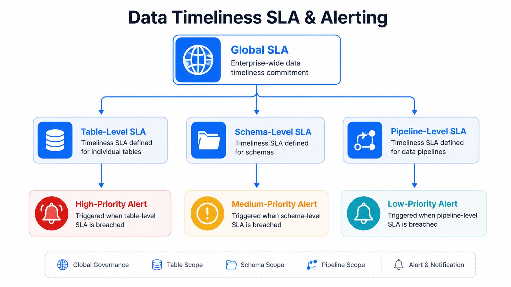
Alert design should reduce noise before it reduces latency. Group related delays, suppress alerts during known maintenance windows, and use confidence ranges instead of binary pass/fail checks where possible. A table-level SLA can trigger a high-priority alert, while a schema-level shift may justify a different escalation path if the arrival window is still intact.
Operational rule: if engineers dismiss an alert twice, the alert design is wrong, not the team.
A practical SLA stack starts at the global policy level, then narrows to table, schema, and pipeline rules. That structure keeps business impact visible without turning every late run into a page at 2 a.m.
Root-Cause Workflows for Late or Missing Data Arrivals
A missed arrival window is a symptom, not a diagnosis. The fastest teams resist the urge to blame the warehouse first. They trace the delay backward, from the table that's late to the system that introduced the lag.
Work from symptom to source
Start with the late dataset and check whether the upstream source was delayed, unavailable, or incomplete. Then inspect orchestration logs for missed schedules, failed retries, or dependency bottlenecks. If the source and scheduler look fine, move into transformation errors and warehouse contention, since both can stall delivery without making the problem obvious at the top of the DAG.
The most useful habit is to compare the current delay against historical observability patterns. If the timing drift is isolated, you probably have an anomaly. If it's getting wider over several runs, you may be looking at a degrading pipeline or a source system that's slowly slipping out of its normal pattern. That is where timing observability pairs well with anomaly detection and schema tracking, because a schema change can break a load without changing the job name.
Use a repeatable investigation checklist
A concise workflow keeps incident response consistent.
Check source system status. Confirm the upstream producer published the expected batch.
Validate pipeline logs. Look for retries, skipped tasks, or orchestration failures.
Inspect transformation errors. Catch silent parsing issues, null explosions, or join breakage.
Review the SLA threshold. Verify the alert wasn't misclassified by an outdated window.
Document findings. Capture the cause, fix, and new guardrail so the same delay doesn't repeat.
The point isn't just speed. It's creating a shared investigation path that reduces mean time to resolution and makes the next incident easier to localize.
In-Database Implementation Tips with digna Timeliness and Analytics
Moving timing checks out of the warehouse adds friction for no good reason. The cleaner pattern is to compute arrival metrics where the data already lives, then surface the results in the same environment that stores the pipeline state. That keeps the data resident in the customer-controlled system and avoids shipping sensitive tables around just to measure freshness.
Wire the checks into the warehouse
The first step is to compute actual arrival timing in-database, then compare it to the learned expected window. digna Timeliness does that by monitoring data arrival against learned patterns and user schedules, including expected delivery time and delay detection. Paired with digna Data Analytics, it can examine historical observability metrics for trends, fast-changing signals, and statistical patterns that help recalibrate the window over time.
I've found this matters most in enterprise warehouses where large tables make external polling awkward and expensive. In-database execution keeps the metric close to the data, which makes the alert path simpler and the operational story easier to trust.
Configure for the pipeline you actually run
Use the same logic for common patterns, but tune the baseline to the table's behavior. For a daily fact table, the expected window should reflect the normal post-cutoff roll. For a volatile feed, the window should be wider and more probabilistic. For a critical downstream model input, pair the timing check with schema tracking and record-level validation so a “late but present” load doesn't hide bad content.
If you want a starting point, the digna Timeliness module is built for arrival monitoring against learned patterns rather than fixed cron assumptions. That matters because production systems don't stay fixed, and neither should the timing model.
Implementation note: keep the timing metric and the alert consumer in the same environment whenever you can. Every extra hop adds latency, failure modes, and confusion.
The strongest pattern is a small loop, compute the timing metric, compare against learned expectation, surface a dashboard signal, and feed the historical measurements back into the baseline. That gives you a system that improves without turning into a hand-maintained rule set.
Building a Sustainable Data Timeliness Practice
Timeliness monitoring works best when it's part of a broader data observability program, not a sidecar alert. Stale reports, broken dashboards, and unreliable AI inputs often start with the same missed arrival. Once expected delivery time becomes a first-class metric, it protects analysts, engineers, and business users at the same time.
A sustainable practice usually starts small. Identify the critical tables first, establish an initial baseline, define SLAs tied to business impact, configure alerting with real severity levels, and then refine the window as patterns become clearer. Add anomaly detection, schema tracking, and record-level validation to the same operating model so one silent break doesn't mask another.
The business case is straightforward. Data that arrives on time supports better decisions, cleaner audits, and fewer fire drills. More importantly, it gives teams a shared language for what “late” actually means, which is the difference between scattered reactions and a real operating standard.
If you want to replace brittle cron checks with learned arrival windows, visit digna and see how its timeliness, analytics, anomaly detection, and validation capabilities work together inside your own warehouse. Start with the tables that matter most, then use the same in-database model to monitor delay risk before stale data reaches the business.