Metrics System Table: Schema, Queries, and Best Practices

A dashboard owner opens the morning report and finds that the numbers haven't changed since two days ago. The pipeline itself shows green, the warehouse is available, and no job has failed. Later, someone discovers that an upstream column changed type, a transformation skipped part of its input, or the latest partition never arrived. The incident wasn't caused by a missing dashboard. It was caused by missing operational evidence.

A metrics system table provides that evidence in a queryable form. Instead of scattering checks across notebooks, shell scripts, warehouse metadata, and external monitoring tools, teams can record table-level and column-level signals in one operational ledger. That ledger can support freshness checks, volume analysis, schema-change detection, historical investigation, ownership workflows, and audit trails without turning every investigation into a custom engineering project.

Table of Contents

• Why Data Teams Need a Metrics System Table

  • The practical gap between collection and action

• What a Metrics System Table Is

  • Why the separation matters

  • Vendor metadata versus a controlled internal ledger

• Core Schema and Column Design Patterns

  • A reference design

  • Keys and access paths

• Practical SQL Queries for Common Observability Tasks

  • Freshness violations

  • Volume anomalies

  • Schema drift

• Retention and Aggregation Strategies

  • Raw-only retention

  • Time-bucketed summaries

  • Tiered retention

• Connecting Metrics to Freshness and Schema Drift Signals

  • Correlating signals

  • A decision matrix for low-noise response

• When More Metrics Reduce Observability Effectiveness

  • Prioritize by consequence

  • Retire checks that don't change decisions

• Instrumenting Metrics Tables in Enterprise Platforms

  • A deployment pattern that holds up

  • Protect performance

• Governance and Auditability in Regulated Industries

  • Separate writers from readers

• Quick Reference for Metrics System Table Design

  • Production query patterns

  • Thresholds need context

Why Data Teams Need a Metrics System Table

A data team usually notices reliability problems through their consumers. An analyst reports that a revenue dashboard is stale. A finance user spots an unexpected change in a report. A machine learning engineer finds that a feature table contains an unfamiliar type or an unusual concentration of missing values. By then, the system has already failed its operational purpose, even if every orchestration task completed successfully.

The missing layer is often a small set of durable observability primitives. A metrics system table can capture row counts, missing-value rates, distinct-value behavior, timestamps, latency, and schema fingerprints at the table or column level. Those values turn an invisible change into a record that SQL can inspect, compare, retain, and route to an owner.

The distinction matters because pipeline status answers only one question: did the task run? It doesn't answer whether the data arrived on schedule, whether the output volume is plausible, whether a critical column changed, or whether a downstream business process can trust the result. A data observability foundation adds those signals to the operational picture.

The practical gap between collection and action

Ad-hoc scripts often work for a first check. They become difficult to govern when every team implements its own naming conventions, thresholds, schedules, and alert destinations. External tools can add coverage, but they may leave metric definitions, historical context, and ownership metadata split across multiple systems.

A centralized table gives engineers a stable interface:

• Detection: store the observed value and the time it was computed.

• Comparison: evaluate it against a baseline, service-level expectation, or prior period.

• Escalation: attach severity, owner, runbook, and status.

• Evidence: preserve what was checked, when it ran, and what result it produced.

Practical rule: A metric isn't operational until someone can query it, identify its owner, decide what action it should trigger, and review its history.

Oracle's metric tables illustrate the architectural shift from manual point-in-time inspection to standardized current and historical tracking. Oracle 10g introduced metric tables that computed deltas and rates, simplifying questions such as the current database I/O rate. Related historical views support trend analysis, including DBA_HIST_SYSMETRIC_SUMMARY for multi-day analysis and DBA_HIST_METRIC_NAME for identifying metrics in a shared AWR repository. Oracle metric-table history and operational tracking shows why the pattern remains useful: teams need both the current state and the evidence needed to understand how that state developed.

Without a metrics system table, teams react to complaints. With one, they can detect degradation before a stakeholder opens a ticket, correlate several signals, and create governance-ready evidence from the same operational record.

What a Metrics System Table Is

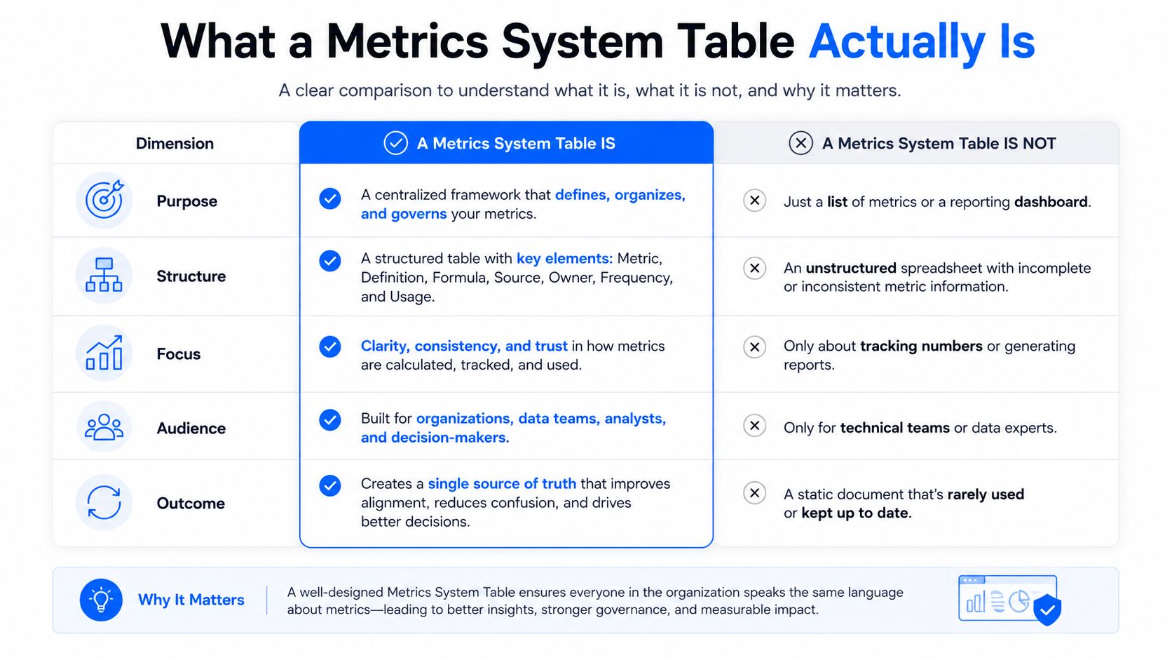
A metrics system table is a low-latency operational ledger of computed observations about data assets. It records measurements derived from user tables, pipelines, or platform metadata without replacing the underlying data or creating a second warehouse copy.

A user-facing table contains business entities such as orders, users, events, or claims. A metrics table records observations about those entities, including a row count at a point in time, latest event timestamp, missing-value ratio, cardinality estimate, schema fingerprint, or validation result. The measured value belongs in the metric record. Source rows remain in the application or analytical table.

Why the separation matters

The two workloads have different shapes. User tables may support transactions, joins, aggregations, or ingestion. A metrics system table is generally designed for time-window queries, filtered lookups, append-oriented writes, and historical comparisons. Treating it like a transactional fact table adds detail, storage, and query overhead without improving operational decisions.

A practical record can include:

• Dimensions: database, schema, table, column, metric type, environment, and business domain.

• Measures: observed value, affected-row count, resource usage, or anomaly score.

• Execution metadata: computation time, source query or job identifier, check version, and result status.

• Governance context: owner, severity, lineage reference, and remediation state.

The table should also support prioritization. A high-volume stream of measurements is not an alerting workflow by itself. Teams need thresholds, ownership, and status fields that let them filter routine variance from conditions requiring action. Keeping those decisions close to the recorded observation supports low-noise, governance-ready operations and allows checks to execute against data in the database rather than exporting every detail elsewhere.

This design fits the role of relational system tables as a metadata layer. They expose profiling and monitoring signals rather than ordinary application rows. A compact, timestamped aggregate can serve as an operational ledger while controlling storage and query overhead, as described in system-table design guidance.

Vendor metadata versus a controlled internal ledger

Snowflake, BigQuery, and Databricks provide system-generated metadata, query history, table history, and information-schema views. These sources help with platform-specific inspection, but they may not provide the retention policy, naming model, business checks, ownership fields, or cross-platform schema an enterprise requires.

A custom table lets a team define:

• which metrics are authoritative,

• how often each metric is computed,

• how long raw and summarized records remain available,

• which thresholds create incidents,

• and which metadata auditors and data stewards can inspect.

That control matters when a freshness result, schema event, or business validation must remain understandable after the original pipeline changes. A semantic layer can standardize business meaning above these signals without hiding the operational record. Teams evaluating that boundary can compare the ledger approach with a dbt semantic layer.

Core Schema and Column Design Patterns

A useful schema separates what was measured, what value was observed, and how the observation was produced. Combining those roles into one overloaded column makes filtering, retention, and alerting harder.

Start with a narrow event model. Static dimensions identify the asset and metric. Dynamic fields store the result at a particular observation time. Execution metadata explains the computation and gives operators enough context to reproduce or triage the result.

A reference design

The exact types vary by platform, but the design principle holds. Use DECIMAL for ratios when precision matters, TIMESTAMP WITH TIME ZONE for observation times, and a structured extension field such as JSONB for evolving details like failure reasons, filter definitions, or source job identifiers. Don't put core filter dimensions inside JSON if operators query them regularly. Promote those fields into indexed columns.

A PostgreSQL-style implementation might look like this:

CREATE TABLE observability.metrics_system (
    table_name       TEXT NOT NULL,
    column_name      TEXT,
    metric_type      TEXT NOT NULL,
    computed_at      TIMESTAMP WITH TIME ZONE NOT NULL,
    metric_value     DECIMAL(38, 12),
    threshold_min    DECIMAL(38, 12),
    threshold_max    DECIMAL(38, 12),
    status           TEXT NOT NULL,
    metadata         JSONB,
    PRIMARY KEY (table_name, column_name, metric_type, computed_at)
);

CREATE TABLE observability.metrics_system (
    table_name       TEXT NOT NULL,
    column_name      TEXT,
    metric_type      TEXT NOT NULL,
    computed_at      TIMESTAMP WITH TIME ZONE NOT NULL,
    metric_value     DECIMAL(38, 12),
    threshold_min    DECIMAL(38, 12),
    threshold_max    DECIMAL(38, 12),
    status           TEXT NOT NULL,
    metadata         JSONB,
    PRIMARY KEY (table_name, column_name, metric_type, computed_at)
);

CREATE TABLE observability.metrics_system (
    table_name       TEXT NOT NULL,
    column_name      TEXT,
    metric_type      TEXT NOT NULL,
    computed_at      TIMESTAMP WITH TIME ZONE NOT NULL,
    metric_value     DECIMAL(38, 12),
    threshold_min    DECIMAL(38, 12),
    threshold_max    DECIMAL(38, 12),
    status           TEXT NOT NULL,
    metadata         JSONB,
    PRIMARY KEY (table_name, column_name, metric_type, computed_at)
);

Keys and access paths

The composite key prevents duplicate observations for the same asset, metric, and computation time. In systems where reruns can produce multiple legitimate results, add a run identifier and make the uniqueness rule reflect that execution model rather than overwriting evidence.

Create access paths around real operator questions:

CREATE INDEX metrics_freshness_recent_idx
ON observability.metrics_system (metric_type, computed_at, table_name)
WHERE metric_type = 'freshness';

CREATE INDEX metrics_asset_time_idx
ON observability.metrics_system (table_name, computed_at);

CREATE INDEX metrics_freshness_recent_idx
ON observability.metrics_system (metric_type, computed_at, table_name)
WHERE metric_type = 'freshness';

CREATE INDEX metrics_asset_time_idx
ON observability.metrics_system (table_name, computed_at);

CREATE INDEX metrics_freshness_recent_idx
ON observability.metrics_system (metric_type, computed_at, table_name)
WHERE metric_type = 'freshness';

CREATE INDEX metrics_asset_time_idx
ON observability.metrics_system (table_name, computed_at);

A query for recent freshness violations can then filter by metric type and time range instead of scanning unrelated checks. MySQL's information-schema guidance makes the same operational point from another angle: dynamic metadata such as row counts, data length, index length, update time, and cardinality can add overhead, so teams should query only the needed objects and avoid broad scans. Information-schema optimization guidance supports filtered access by schema, table, metric type, and time window.

The schema should also be documented alongside the checks that populate it. A warehouse schema catalog can help teams reason about dependencies, but the metrics ledger should remain optimized for operational access, not descriptive completeness. See schemas in a data warehouse for the boundary between structural metadata and monitoring evidence.

Practical SQL Queries for Common Observability Tasks

SQL becomes useful when each query answers an operational question and returns enough context for a decision. The following patterns assume the reference table from the previous section and use PostgreSQL-style syntax. Snowflake, BigQuery, and Redshift require small changes to timestamp, percentile, and date-function syntax.

Freshness violations

Store the latest observed source timestamp as metric_value for a freshness metric, or store it in structured metadata if the platform needs a separate numeric age value. The query below compares the newest observation with an SLA stored in a configuration table.

WITH latest AS (
    SELECT
        table_name,
        MAX(computed_at) AS last_observed_at
    FROM observability.metrics_system
    WHERE metric_type = 'freshness'
      AND computed_at >= CURRENT_TIMESTAMP - INTERVAL '1 day'
    GROUP BY table_name
)
SELECT
    table_name,
    last_observed_at,
    CURRENT_TIMESTAMP - last_observed_at AS age,
    c.max_age
FROM latest
JOIN observability.metric_config AS c
  ON c.table_name = latest.table_name
WHERE CURRENT_TIMESTAMP - last_observed_at > c.max_age;

WITH latest AS (
    SELECT
        table_name,
        MAX(computed_at) AS last_observed_at
    FROM observability.metrics_system
    WHERE metric_type = 'freshness'
      AND computed_at >= CURRENT_TIMESTAMP - INTERVAL '1 day'
    GROUP BY table_name
)
SELECT
    table_name,
    last_observed_at,
    CURRENT_TIMESTAMP - last_observed_at AS age,
    c.max_age
FROM latest
JOIN observability.metric_config AS c
  ON c.table_name = latest.table_name
WHERE CURRENT_TIMESTAMP - last_observed_at > c.max_age;

WITH latest AS (
    SELECT
        table_name,
        MAX(computed_at) AS last_observed_at
    FROM observability.metrics_system
    WHERE metric_type = 'freshness'
      AND computed_at >= CURRENT_TIMESTAMP - INTERVAL '1 day'
    GROUP BY table_name
)
SELECT
    table_name,
    last_observed_at,
    CURRENT_TIMESTAMP - last_observed_at AS age,
    c.max_age
FROM latest
JOIN observability.metric_config AS c
  ON c.table_name = latest.table_name
WHERE CURRENT_TIMESTAMP - last_observed_at > c.max_age;

Partition the table by computed_at where the platform supports it. The bounded time predicate enables partition pruning and prevents an all-history scan.

Volume anomalies

A rolling baseline should reflect normal variation rather than a single prior run. This example uses a rolling average and standard deviation over historical row-count metrics.

WITH history AS (
    SELECT
        table_name,
        computed_at,
        metric_value AS row_count,
        AVG(metric_value) OVER (
            PARTITION BY table_name
            ORDER BY computed_at
            ROWS BETWEEN 7 PRECEDING AND 1 PRECEDING
        ) AS rolling_avg,
        STDDEV_SAMP(metric_value) OVER (
            PARTITION BY table_name
            ORDER BY computed_at
            ROWS BETWEEN 7 PRECEDING AND 1 PRECEDING
        ) AS rolling_stddev
    FROM observability.metrics_system
    WHERE metric_type = 'row_count'
      AND computed_at >= CURRENT_TIMESTAMP - INTERVAL '30 days'
)
SELECT *
FROM history
WHERE rolling_avg IS NOT NULL
  AND (
      row_count > rolling_avg + (2 * rolling_stddev)
      OR row_count < rolling_avg - (2 * rolling_stddev)
  );

WITH history AS (
    SELECT
        table_name,
        computed_at,
        metric_value AS row_count,
        AVG(metric_value) OVER (
            PARTITION BY table_name
            ORDER BY computed_at
            ROWS BETWEEN 7 PRECEDING AND 1 PRECEDING
        ) AS rolling_avg,
        STDDEV_SAMP(metric_value) OVER (
            PARTITION BY table_name
            ORDER BY computed_at
            ROWS BETWEEN 7 PRECEDING AND 1 PRECEDING
        ) AS rolling_stddev
    FROM observability.metrics_system
    WHERE metric_type = 'row_count'
      AND computed_at >= CURRENT_TIMESTAMP - INTERVAL '30 days'
)
SELECT *
FROM history
WHERE rolling_avg IS NOT NULL
  AND (
      row_count > rolling_avg + (2 * rolling_stddev)
      OR row_count < rolling_avg - (2 * rolling_stddev)
  );

WITH history AS (
    SELECT
        table_name,
        computed_at,
        metric_value AS row_count,
        AVG(metric_value) OVER (
            PARTITION BY table_name
            ORDER BY computed_at
            ROWS BETWEEN 7 PRECEDING AND 1 PRECEDING
        ) AS rolling_avg,
        STDDEV_SAMP(metric_value) OVER (
            PARTITION BY table_name
            ORDER BY computed_at
            ROWS BETWEEN 7 PRECEDING AND 1 PRECEDING
        ) AS rolling_stddev
    FROM observability.metrics_system
    WHERE metric_type = 'row_count'
      AND computed_at >= CURRENT_TIMESTAMP - INTERVAL '30 days'
)
SELECT *
FROM history
WHERE rolling_avg IS NOT NULL
  AND (
      row_count > rolling_avg + (2 * rolling_stddev)
      OR row_count < rolling_avg - (2 * rolling_stddev)
  );

Use a partition or clustering key on table name and observation time. The exact band should reflect business risk and seasonality, not a universal constant.

Schema drift

Schema drift is easiest to detect when a baseline snapshot is stored as a distinct metric family. The query below compares the current schema fingerprint detail with the last approved snapshot.

WITH current_schema AS (
    SELECT
        table_name,
        column_name,
        metadata ->> 'data_type' AS data_type
    FROM observability.metrics_system
    WHERE metric_type = 'schema_snapshot'
      AND computed_at = (
          SELECT MAX(computed_at)
          FROM observability.metrics_system
          WHERE metric_type = 'schema_snapshot'
      )
),
baseline AS (
    SELECT table_name, column_name, data_type
    FROM observability.schema_baseline
)
SELECT
    COALESCE(c.table_name, b.table_name) AS table_name,
    COALESCE(c.column_name, b.column_name) AS column_name,
    b.data_type AS baseline_type,
    c.data_type AS current_type,
    CASE
        WHEN b.column_name IS NULL THEN 'added'
        WHEN c.column_name IS NULL THEN 'dropped'
        WHEN b.data_type <> c.data_type THEN 'type_changed'
    END AS drift_type
FROM current_schema AS c
FULL OUTER JOIN baseline AS b
  ON c.table_name = b.table_name
 AND c.column_name = b.column_name
WHERE b.column_name IS NULL
   OR c.column_name IS NULL
   OR b.data_type <> c.data_type;

WITH current_schema AS (
    SELECT
        table_name,
        column_name,
        metadata ->> 'data_type' AS data_type
    FROM observability.metrics_system
    WHERE metric_type = 'schema_snapshot'
      AND computed_at = (
          SELECT MAX(computed_at)
          FROM observability.metrics_system
          WHERE metric_type = 'schema_snapshot'
      )
),
baseline AS (
    SELECT table_name, column_name, data_type
    FROM observability.schema_baseline
)
SELECT
    COALESCE(c.table_name, b.table_name) AS table_name,
    COALESCE(c.column_name, b.column_name) AS column_name,
    b.data_type AS baseline_type,
    c.data_type AS current_type,
    CASE
        WHEN b.column_name IS NULL THEN 'added'
        WHEN c.column_name IS NULL THEN 'dropped'
        WHEN b.data_type <> c.data_type THEN 'type_changed'
    END AS drift_type
FROM current_schema AS c
FULL OUTER JOIN baseline AS b
  ON c.table_name = b.table_name
 AND c.column_name = b.column_name
WHERE b.column_name IS NULL
   OR c.column_name IS NULL
   OR b.data_type <> c.data_type;

WITH current_schema AS (
    SELECT
        table_name,
        column_name,
        metadata ->> 'data_type' AS data_type
    FROM observability.metrics_system
    WHERE metric_type = 'schema_snapshot'
      AND computed_at = (
          SELECT MAX(computed_at)
          FROM observability.metrics_system
          WHERE metric_type = 'schema_snapshot'
      )
),
baseline AS (
    SELECT table_name, column_name, data_type
    FROM observability.schema_baseline
)
SELECT
    COALESCE(c.table_name, b.table_name) AS table_name,
    COALESCE(c.column_name, b.column_name) AS column_name,
    b.data_type AS baseline_type,
    c.data_type AS current_type,
    CASE
        WHEN b.column_name IS NULL THEN 'added'
        WHEN c.column_name IS NULL THEN 'dropped'
        WHEN b.data_type <> c.data_type THEN 'type_changed'
    END AS drift_type
FROM current_schema AS c
FULL OUTER JOIN baseline AS b
  ON c.table_name = b.table_name
 AND c.column_name = b.column_name
WHERE b.column_name IS NULL
   OR c.column_name IS NULL
   OR b.data_type <> c.data_type;

Teams that want to measure schema drift operationally can track drift frequency and drift detection latency, defined as the number of schema changes in a period and the time between a change and its detection. Schema-drift monitoring guidance describes those measures without requiring every structural change to become an incident.

Keep these queries version-controlled and review them like production code. SQL query optimization practices are especially relevant when the metrics table contains months of observations.

Retention and Aggregation Strategies

Raw observations are valuable during incident response and expensive when retained without a plan. A metrics table that records every run, asset, and check can grow quickly, so retention should match the questions operators need to answer.

Three patterns cover most deployments.

Raw-only retention

This model keeps detailed records and prunes them with a time-to-live policy. It preserves the best forensic detail, including exact execution context and the sequence of changes that preceded an incident. The downside is that historical trend queries scan more rows, and the table needs disciplined partition maintenance.

Raw-only retention works when incident investigation is the dominant use case or when the platform already provides inexpensive partition pruning. It works poorly when governance teams need long historical trends and operators routinely query the whole table.

Time-bucketed summaries

Hourly or daily rollups store aggregates such as minimum, maximum, average, count, latest value, and anomaly count. They make trend analysis faster and reduce the amount of historical data that must remain in the hot warehouse. The trade-off is irreversibility. A daily summary can show that a table behaved abnormally, but it may not reveal which run, column, or check produced the first deviation.

Use materialized views or incremental dbt models for these summaries. Partition by the bucket date, and keep the dimensions required for the most common filters, such as table, metric type, domain, and environment.

Tiered retention

A hybrid model keeps raw records for a short operational window and rolled-up summaries for a longer analytical window. It balances incident detail with trend visibility, while cold storage can hold compliance evidence when interactive query latency isn't required.

Retention decision: Keep raw detail where it changes the outcome of an investigation. Roll up records when the remaining question is directional, comparative, or governance-focused.

Align retention with access patterns. If operators filter by table and recent time, partition on observation date and cluster or index by table name. If auditors filter by control, owner, or reporting period, preserve those fields in the summary rather than forcing them to reconstruct context from raw events.

Historical warehouse features can complement this design, but they don't remove the need to choose which metric records remain queryable. Snowflake historical data patterns provide useful context for separating operational history from long-term analysis.

Connecting Metrics to Freshness and Schema Drift Signals

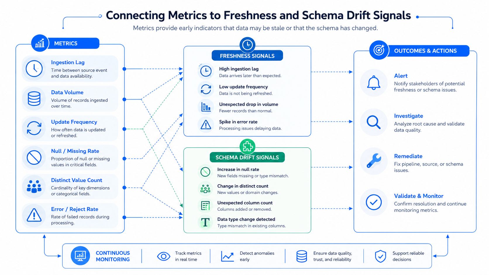
A single metric rarely explains whether a table is safe to consume. A late arrival may be harmless if the source schedule changed. A row-count shift may be expected during a seasonal event. A schema change may be backward-compatible. The useful signal appears when several observations point to the same failure mode.

Freshness, volume, and schema records can be joined by table identifier and a common time window. From there, teams can build a composite reliability index, but the score should rank investigation priority rather than pretend to represent an objective truth.

Correlating signals

A simple correlation query can identify tables with multiple simultaneous conditions:

WITH signals AS (
    SELECT
        table_name,
        MAX(CASE WHEN metric_type = 'freshness' AND status = 'fail' THEN 1 ELSE 0 END) AS freshness_fail,
        MAX(CASE WHEN metric_type = 'row_count' AND status = 'fail' THEN 1 ELSE 0 END) AS volume_fail,
        MAX(CASE WHEN metric_type = 'schema_snapshot' AND status = 'fail' THEN 1 ELSE 0 END) AS schema_fail
    FROM observability.metrics_system
    WHERE computed_at >= CURRENT_TIMESTAMP - INTERVAL '1 hour'
    GROUP BY table_name
)
SELECT
    table_name,
    freshness_fail,
    volume_fail,
    schema_fail,
    freshness_fail + volume_fail + schema_fail AS failed_signal_count
FROM signals
WHERE freshness_fail + volume_fail + schema_fail >= 2;

WITH signals AS (
    SELECT
        table_name,
        MAX(CASE WHEN metric_type = 'freshness' AND status = 'fail' THEN 1 ELSE 0 END) AS freshness_fail,
        MAX(CASE WHEN metric_type = 'row_count' AND status = 'fail' THEN 1 ELSE 0 END) AS volume_fail,
        MAX(CASE WHEN metric_type = 'schema_snapshot' AND status = 'fail' THEN 1 ELSE 0 END) AS schema_fail
    FROM observability.metrics_system
    WHERE computed_at >= CURRENT_TIMESTAMP - INTERVAL '1 hour'
    GROUP BY table_name
)
SELECT
    table_name,
    freshness_fail,
    volume_fail,
    schema_fail,
    freshness_fail + volume_fail + schema_fail AS failed_signal_count
FROM signals
WHERE freshness_fail + volume_fail + schema_fail >= 2;

WITH signals AS (
    SELECT
        table_name,
        MAX(CASE WHEN metric_type = 'freshness' AND status = 'fail' THEN 1 ELSE 0 END) AS freshness_fail,
        MAX(CASE WHEN metric_type = 'row_count' AND status = 'fail' THEN 1 ELSE 0 END) AS volume_fail,
        MAX(CASE WHEN metric_type = 'schema_snapshot' AND status = 'fail' THEN 1 ELSE 0 END) AS schema_fail
    FROM observability.metrics_system
    WHERE computed_at >= CURRENT_TIMESTAMP - INTERVAL '1 hour'
    GROUP BY table_name
)
SELECT
    table_name,
    freshness_fail,
    volume_fail,
    schema_fail,
    freshness_fail + volume_fail + schema_fail AS failed_signal_count
FROM signals
WHERE freshness_fail + volume_fail + schema_fail >= 2;

The escalation rule should reflect consequence. A freshness failure plus a volume failure may justify an automated retry or source investigation. A schema change combined with a type-sensitive downstream model should pause promotion and request steward review. An isolated null-rate fluctuation may need observation rather than paging.

A decision matrix for low-noise response

Schema drift monitoring asks whether a column was added, removed, or retyped without warning. Freshness asks whether data is arriving on schedule. Those definitions are operationally distinct, and data observability signal guidance is useful when designing the metric taxonomy.

Teams can execute these checks directly inside the database, avoiding unnecessary data movement and reducing the distance between observation and decision. In-database observability execution describes this model as running tests directly within the database environment, which fits a metrics system table that stores compact results rather than extracted source data.

When More Metrics Reduce Observability Effectiveness

Coverage sounds safe until the metric table becomes a catalogue of everything that can be measured. At that point, query costs rise, alert streams become difficult to classify, and important failures compete with harmless fluctuations.

A team can track a large set of column-level statistics while missing a business logic failure. It can also produce so many notifications that engineers acknowledge them without investigation. The problem isn't measurement itself. The problem is treating every measurement as equally actionable.

Prioritize by consequence

Start with the signals that affect a consumer's ability to use the data:

• Tier-one freshness: Monitor whether executive, regulatory, customer-facing, or operational tables arrive when expected.

• Table-level volume: Detect empty loads, partial extracts, and unexpected source changes before adding granular checks.

• Schema compatibility: Apply structural monitoring to critical paths where a type or column change can break models.

• Targeted column checks: Add null-rate, cardinality, or distribution checks when a specific column influences a financial calculation, model feature, or compliance control.

This sequence keeps the metrics system table an operational ledger, not a full data catalogue. Broader table-level monitoring can cover freshness, schema drift, and volume anomalies without requiring hundreds of rules for every dataset, while deeper validation remains available for high-risk assets. Unified data-quality and observability guidance supports that layered approach.

Retire checks that don't change decisions

Every check should have an owner, a response, and a reason to remain active. If a metric has produced no actionable response over its review period, ask whether the threshold is wrong, the asset is low priority, or the check no longer belongs in continuous monitoring.

Operational test: If an alert can't identify a responsible team and a next action, it probably shouldn't page anyone.

Use dashboards for exploratory context and alerts for decisions. A table-level freshness violation may page an owner. A small distribution movement may remain visible in trend analysis until it combines with another signal. Snowflake's discussion of data-quality remediation reinforces the broader trade-off: monitoring coverage is useful only when teams can act on the result, not when it produces more unreviewed output. See data-quality fixing workflows.

The right target isn't maximum metric volume. It's the smallest set of signals that detects meaningful degradation early, supports diagnosis, and creates a defensible record of what happened.

Instrumenting Metrics Tables in Enterprise Platforms

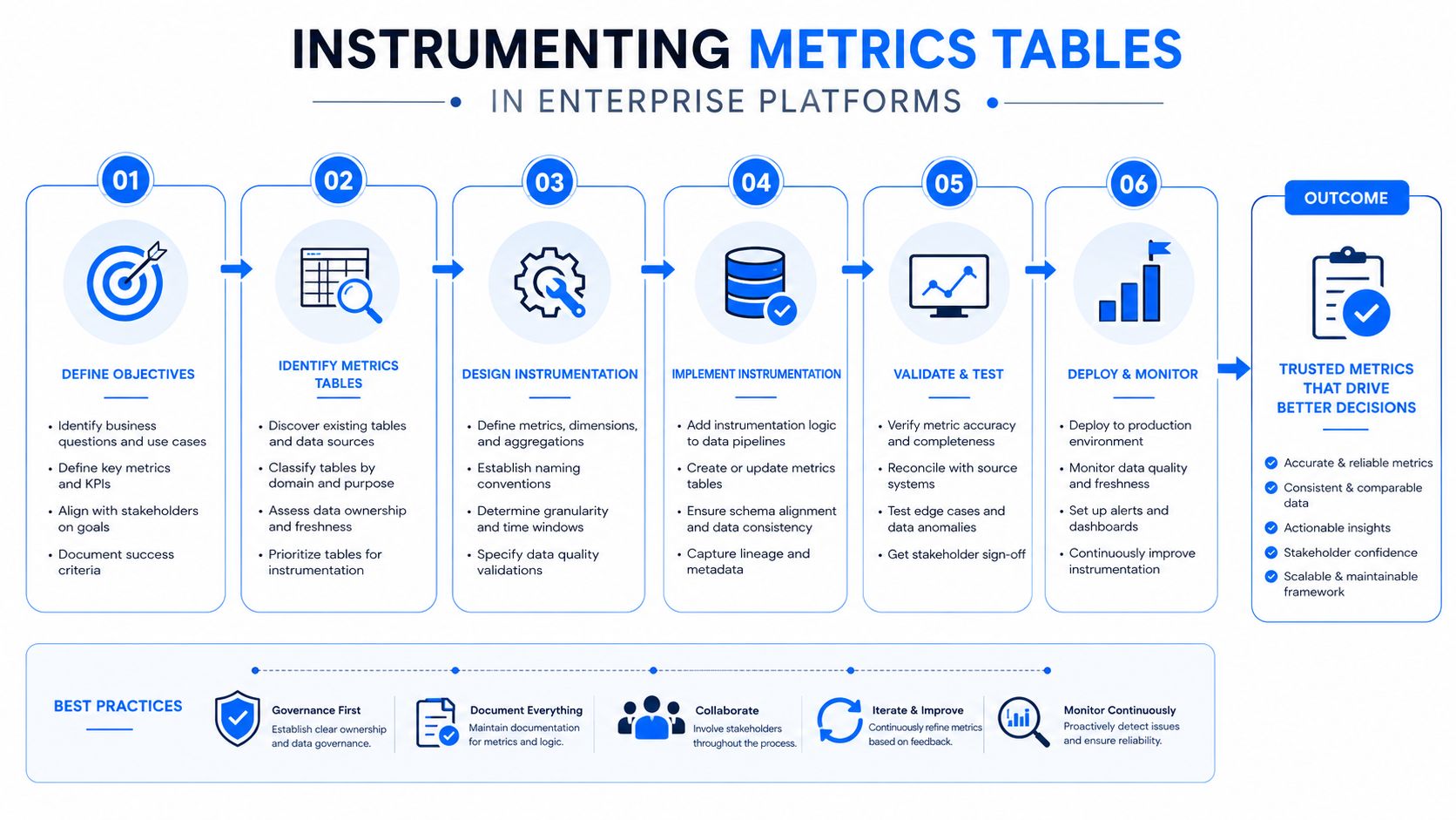
Production instrumentation should run close to the data and live in version control. Scheduled SQL tasks, dbt post-hooks, warehouse-native procedures, and platform orchestration can populate a metrics system table without exporting raw records to a separate service.

The implementation choice depends on the check. A freshness query can run after ingestion. A schema snapshot can run before downstream models are released. A heavier distribution calculation may run on a schedule that matches its risk and cost. The important point is that the schedule, query, threshold, owner, and retention policy should be declared together.

A deployment pattern that holds up

1. Create the ledger. Add the metric table, configuration table, ownership fields, and retention mechanism before enabling alerts.

2. Register critical assets. Record table identifiers, business domain, severity, expected schedule, and responsible team.

3. Populate from the database. Use scheduled SQL, dbt hooks, or native tasks to compute compact aggregates in place.

4. Baseline before paging. Store observations long enough to understand normal behavior, then set thresholds that reflect the asset.

5. Route actionable results. Push approved incidents to Slack, PagerDuty, governance dashboards, or an existing observability tool.

6. Attach runbooks. Store remediation references with the metric configuration so an alert opens with context.

A platform such as Monte Carlo can consume warehouse signals, while a custom service can query the ledger directly. digna provides in-database metric computation for record counts, missing-value rates, distribution statistics, KPI aggregations, and timeliness deviations, with modules for anomaly detection, validation, and schema tracking.

Protect performance

Index or cluster on the fields operators filter most often. Partition by observation date where supported. Avoid recalculating expensive metrics for every table on every run, and don't let an alert query scan all historical records when a recent partition contains the necessary evidence.

Keep check definitions in a repository and review changes through the same process as transformation code. Notebook logic and scattered scripts are difficult to audit, reproduce, or retire. A versioned configuration makes ownership changes, threshold edits, and schema evolution visible.

Governance and Auditability in Regulated Industries

In finance, healthcare, telecommunications, and the public sector, observability evidence must survive beyond the incident that created it. A metrics system table can record that a check ran, what it measured, which version executed, whether it passed, and who owned the result.

That record supports more than incident response. It can help an auditor verify that a critical financial table was validated before a reporting process, or that a sensitive column remained within its expected quality range. The value comes from preserving execution evidence and making the evidence explainable.

Separate writers from readers

Automated pipelines should own writes. Auditors, data stewards, control owners, and platform engineers should receive scoped read access. Avoid giving operational users permission to edit historical results, because mutable evidence weakens the audit trail.

Useful audit fields include:

• check_executed_at, the time the evaluation ran.

• observed_at, the time represented by the metric.

• check_version, identifying the logic used.

• owner_team, identifying accountability.

• lineage_reference, connecting the result to upstream and downstream assets.

• result_status and failure_reason, making the outcome understandable.

• remediation_status, showing whether the issue was reviewed or resolved.

Regulated retention can extend well beyond the hot-query window. Store recent evidence in the warehouse for operational access, compress older partitions, and archive immutable records to controlled object storage when interactive access is no longer necessary. Apply encryption, access logging, and deletion policies that match the governing data classification.

A metrics system table becomes governance infrastructure when its records are immutable, attributable, reproducible, and connected to the underlying data lineage. It shouldn't merely say that a check failed. It should explain which check ran, against which asset, under which definition, and what happened afterward.

Quick Reference for Metrics System Table Design

A production design should be easy to inspect during an incident. The table below condenses the fields that usually matter most.

Production query patterns

• Freshness checks: Filter recent metric_type = 'freshness' records and compare the latest observation with the asset's configured age limit.

• Volume anomalies: Use a bounded historical window, window functions, and a table-specific baseline rather than comparing every result with the immediately previous run.

• Schema drift alerts: Compare the current schema snapshot with an approved baseline and classify additions, removals, and type changes separately.

• Null-rate monitors: Filter by column and metric type, then evaluate the current ratio against the column's expected range.

• Latency trackers: Use LAG over ordered observations to calculate inter-run gaps and isolate delayed deliveries.

Production-ready filters should narrow by table_name, metric_type, and observation window before applying calculations. That combination supports partition pruning, index use, and lower investigation cost.

Thresholds need context

There is no universal freshness SLA, volume band, or null-rate boundary that fits every enterprise table. A tier-one table may need a tighter delivery expectation than an exploratory dataset. A daily source may tolerate a different volume pattern from a high-frequency event stream. A schema change may be harmless for one consumer and release-blocking for another.

Use historical behavior to establish a baseline, then combine thresholds with consequence and ownership. Require multiple related signals before escalating noisy conditions, and keep the alert record rich enough to support a handoff. Review checks regularly, remove measurements that don't lead to action, and retain the underlying evidence required for governance.

digna helps teams compute and analyze table-level metrics in-database, monitor timeliness and anomalies, validate records, and track schema changes without moving production data out of the customer environment. Visit digna to see how its modular observability capabilities can turn a metrics system table into a governed workflow for data engineers, stewards, and platform owners.