What Is the Monte Carlo Simulation
|
7
minuto de lectura

You're in a meeting with a deadline, a dashboard is wobbling, and someone asks for a single number. The platform owner wants a forecast for pipeline latency, the finance lead needs a budget view for a launch, and the logistics manager is staring at traffic, weather, and dock delays. A single estimate feels tidy, but it hides the part that matters most: the spread of plausible outcomes.
Monte Carlo simulation is the method that turns that one guess into a distribution of futures. It does that by replacing certainty with repeated random sampling, then letting the results show what's likely, what's risky, and what's just noise. That's why it keeps showing up in finance, engineering, and enterprise data systems that have to make decisions under uncertainty.
Table of Contents
A Question You Already Need Monte Carlo For
Why that changes the conversation
The Core Idea Behind the Monte Carlo Simulation
The math without the fog
How a Monte Carlo Simulation Actually Runs
The four steps in plain language
Monte Carlo Versus Closed-Form and Sensitivity Analysis
A quick decision rule
Where Monte Carlo Simulation Shows Up in Real Work
The four places it earns its keep
Honest Trade-Offs and Common Pitfalls
The pitfalls that quietly distort results
A notebook checklist that keeps you honest
From Monte Carlo Ideas to Enterprise Data Observability With digna
Why the Monte Carlo lens fits observability
What a team can do first
A Question You Already Need Monte Carlo For
A platform team owner gets asked for end-of-month latency during a leadership review, but the team only has two weeks of noisy history. A finance lead has to defend whether a product launch stays inside budget while ad spend and supplier lead times keep shifting. A logistics manager needs an expected delivery time when traffic, weather, and dock availability all move at once. In each case, a single guess sounds confident and is probably wrong.
The trap is that the guess collapses the whole problem into one number. It says nothing about how often things drift late, how bad the late cases get, or whether the outcome is stable enough to trust. A Monte Carlo simulation replaces that one number with thousands of plausible futures, all drawn from the same uncertainty.
Why that changes the conversation
Once you see a distribution instead of a point estimate, the question changes. You stop asking, “What's the answer?” and start asking, “How wide is the risk band, and what drives it?” That's a better question for budgets, schedules, and operational SLAs.
The method is simple to describe, even if the modeling takes care. You define the uncertain inputs, sample from them many times, compute the result each time, and summarize the spread. If you want a related primer on how raw data distributions feed that thinking, the distribution of data matters before any simulation is trustworthy.
A Monte Carlo model doesn't promise certainty. It gives you a more honest picture of the uncertainty you already have.
The Core Idea Behind the Monte Carlo Simulation
A good mental model starts with a dartboard. Drop random points on a square, count how many land inside the circle, and use that ratio to estimate π. That's the heart of Monte Carlo thinking, repeated random trials can reveal something hard to calculate directly. The early history of the method includes precursor ideas like Buffon's needle from the 18th century, then systematic use in the 20th century for hard integration and uncertainty problems PMC review.
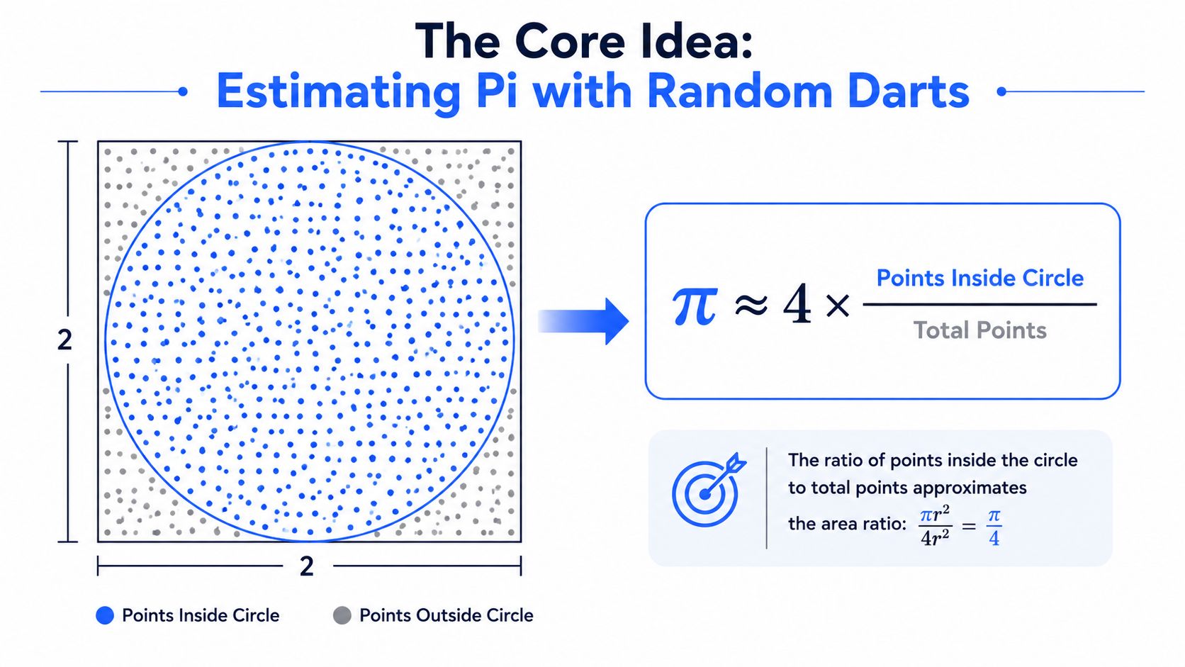
At the modern technical level, Monte Carlo simulation means estimating an expectation, written plainly as E[f(X)], by drawing many random samples of the uncertain inputs X, evaluating the function f each time, and averaging the results. That's the same core idea used in finance, engineering, reliability analysis, and the physical and social sciences, where the computer runs thousands or millions of trials to study variability PMC review.
The math without the fog
You don't need a closed-form formula for the whole system. You only need two things, a way to sample the inputs and a way to compute the output for each trial. That's why Monte Carlo is so useful for nonlinear models and messy real-world systems, the method doesn't depend on elegant algebra to work.
The Law of Large Numbers says the average of the simulated outcomes moves toward the true expectation as the sample size grows. The Central Limit Theorem gives the practical reason this feels stable, the standard error shrinks roughly with the square root of sample size. MIT's finance lecture notes make the scaling plain, direct estimation error tends to fall at about σ/√n, which is why precision improves slowly as you add more runs MIT OCW.
Practical rule: if your problem can be sampled and evaluated, Monte Carlo can usually estimate it, even when exact algebra becomes awkward or impossible.
That generality is the point. The method exists because many real systems refuse to collapse into a neat formula.
How a Monte Carlo Simulation Actually Runs
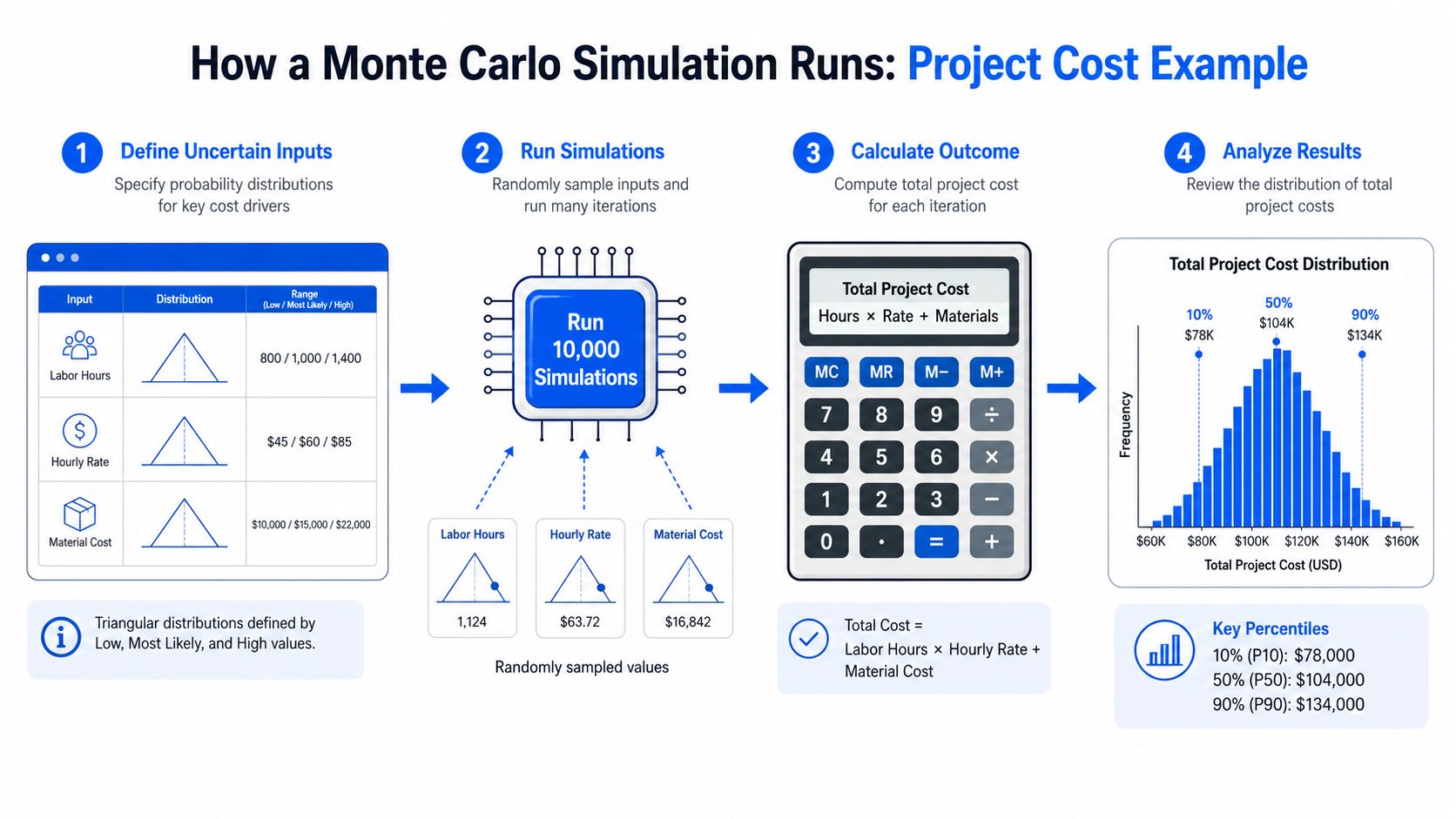
A practical example makes the loop easier to see. Suppose you're estimating total project cost and the uncertain pieces are labor hours, hourly rate, and material cost. You don't know one of those inputs exactly, so you describe each one as a probability distribution instead of a fixed value, often using historical data, expert judgment, or both.
The four steps in plain language
First, define the inputs and choose distributions that match them. A triangular distribution is common in project work because people often know a low, likely, and high estimate even if they don't know a perfectly measured curve.
Second, sample one value from each input distribution to build a single scenario. That one scenario becomes one possible world, and you compute the output, here the total cost.
Third, repeat the draw-and-evaluate loop many times. Modern teaching and research sources describe this as a computer-driven experimental method that can generate thousands or millions of random trials to study distributions and risk PMC review.
Fourth, summarize the output list as its own distribution. You might look at the mean, median, histogram, and the percentiles that matter for a decision, because those tell you how the cost behaves across the full range of plausible outcomes.
Operational habit: watch the running mean while the simulation is executing. If it keeps moving, you probably haven't run enough trials for the estimate to settle.
A simple pseudocode sketch looks like this:
A minimal Python version is just as direct:
For a deeper look at how data assumptions are shaped before a model runs, the statistical methods for data analysis page is a useful companion. The key implementation question is convergence, when more samples stop changing the answer in a material way, you've usually reached a usable stopping point.
Monte Carlo Versus Closed-Form and Sensitivity Analysis
A project-cost model can be attacked three different ways, and each one answers a different question. Closed-form math gives a direct solution when the formulas are tractable. Sensitivity analysis perturbs one variable at a time to see which assumption drives the result. Monte Carlo simulation runs many full scenarios and returns the spread of outcomes, including the chance of budget overrun.
Dimension | Closed-Form Math | Sensitivity Analysis | Monte Carlo Simulation |
|---|---|---|---|
Main question | What's the exact answer? | Which input matters most? | What outcomes are plausible, and how often? |
Inputs | Fixed formulas, often exact | One variable changes at a time | Many uncertain inputs vary together |
Output | Single number or exact expression | Ranked influence or direction of change | Full distribution of outcomes |
Best use | Linear, tractable models | Isolating drivers | Risk, tail behavior, interacting uncertainty |
Weak spot | Breaks down when the math gets messy | Misses interactions | Needs sampling, validation, and compute |
Closed-form math is efficient when the model is simple enough. Sensitivity analysis is useful when you need to know which assumption to fix first. Monte Carlo is the right hammer when uncertainty comes from many interacting inputs, correlations matter, or the model is nonlinear.
A clean way to think about it is the tradeoff between bias and variance. A deterministic shortcut can be neat but misleading, while a richer simulation can capture more of reality if the inputs are sound.
A quick decision rule
If you only need a rough direction, sensitivity analysis may be enough. If the model has a closed form and the inputs are stable, use the exact math. If the outcome depends on many uncertain drivers and the decision hinges on the tail, Monte Carlo earns its compute.
For teams building data workflows, the same logic applies to anomaly review. The outlier identification methods page is relevant when a single bad point can mislead an otherwise healthy model.
Where Monte Carlo Simulation Shows Up in Real Work
The strongest use cases all share the same shape, the decision depends on the tail, not just the mean. In finance, Monte Carlo supports Value-at-Risk on portfolios of correlated assets, because the joint behavior of those assets drives the downside. In engineering, it helps with reliability analysis when different components fail at different rates, so the system view matters more than any single part.

The four places it earns its keep
In timeliness planning, a Monte Carlo model can estimate the probability of breaching an SLA when every stage in the pipeline has jitter. That is more useful than a single estimated arrival time, because operators need to know how likely the bad cases are.
In data observability, the same idea appears in anomaly detection. A platform can treat freshness, volume, and schema signals as uncertain inputs, sample plausible metric states, and estimate whether an alert reflects a real incident or just noise. That's a natural fit for digna's Monte Carlo-style anomaly work, and the spotting data anomalies in your data platform with Monte Carlo simulations page fits that use case.
In supply chain and energy planning, the pattern repeats. Demand uncertainty, inventory risk, and load forecasting all become easier to reason about once the model returns a range of likely outcomes instead of a single optimistic forecast.
If the decision changes when the tail changes, a point estimate is usually too thin to trust.
There's also an important systems lesson here. Monte Carlo isn't only for finance quants or scientists. Any team that has to answer, “What happens when several uncertain things move together?” is already in Monte Carlo territory.
Honest Trade-Offs and Common Pitfalls
Monte Carlo is powerful, but it's not magic. The most important limitation is the slow error scaling, direct estimation error drops with σ/√n, so cutting error in half costs a lot more compute than people expect MIT OCW. That's why variance reduction methods matter, they reduce estimator variance without changing its expected value, which gives you a tighter interval for the same CPU budget Frontiers in Physics.
The pitfalls that quietly distort results
The first trap is input quality. If the distributions don't reflect reality, the simulation just produces a more polished wrong answer. A Gaussian tail can look reassuring in a risk model while the actual world is much fatter-tailed.
The second trap is correlation blindness. Beginners often sample inputs independently because it's easier, then get outcomes that are too smooth and too favorable. That mistake is especially costly in portfolio work, reliability models, and any system where shared drivers move together.
The third trap is convergence that only looks good by eye. A running mean that settles visually can still hide instability in the tail, so you need a stopping rule, not just a hunch.
The fourth trap is silent variance from rare events. If the event you care about happens infrequently, too few runs can miss it entirely, which makes the output look safer than it is. Monte Carlo can understate extremes when the chosen distributions are too tame, especially in finance and systemic risk contexts Analytica on Monte Carlo in finance.
A notebook checklist that keeps you honest
Validate each input against historical data or domain judgment before you simulate.
Include correlation where shared drivers move together.
Pick a stopping rule based on the stability of the result, not just an arbitrary run count.
Report a confidence band, not only a single answer.
Treat the model as one assumption set among several, not as a final truth.
The guide to ETL migration strategies is a useful reminder that downstream data systems also depend on assumption quality. If the upstream shape is wrong, the downstream answer is noisy no matter how elegant the calculation looks.
From Monte Carlo Ideas to Enterprise Data Observability With digna
In enterprise observability, the Monte Carlo mindset shows up as baseline learning and probabilistic alerting. digna watches tables, pipelines, freshness patterns, and business metrics inside the customer's own environment, then learns what normal behavior looks like without forcing teams to hard-code brittle rules. That matters because data doesn't just arrive, it arrives with variation, seasonality, and occasional misses.
Why the Monte Carlo lens fits observability
The useful move is to treat expected freshness, row counts, and null rates as distributions, not fixed thresholds. Once a platform learns that baseline, it can compare live values against the learned range and estimate whether the current state is unusual. That's the same logic Monte Carlo uses in other domains, repeated sampling to understand the spread of plausible outcomes.
The practical loop is easy to follow. digna learns a freshness baseline from historical arrival behavior, samples expected delay states from that learned distribution, and then scores the current observation against those states to decide whether the latency looks anomalous. The result is a confidence-oriented signal, not just a yes/no alarm.
That approach fits naturally with migration and pipeline change work. If a team is moving data flows or reworking sources, the guide to ETL migration strategies gives the surrounding operational context, while Monte Carlo-style observability helps judge whether the new behavior is drifting.
What a team can do first
Turn on baseline learning for critical dashboards and pipelines so the system knows normal behavior before it flags exceptions.
Compare observed distributions against static threshold alerts, because thresholds alone miss variation.
Use confidence bands to rank on-call investigation, so the noisiest signals don't dominate the queue.
For teams that want a single place to connect those ideas, the Monte Carlo data alternative for enterprise data observability page shows how this pattern maps to operational monitoring.
The broader point is simple. Monte Carlo thinking helps you ask a better question, “How likely is this state to be real?” In observability, that question often matters more than whether a metric crossed one fixed line.
If you're trying to make data reliability decisions with less guesswork, visit digna and see how baseline learning, timeliness monitoring, and anomaly detection work together in the same observability platform. It's a practical way to apply Monte Carlo-style uncertainty thinking to pipelines, dashboards, and business metrics that can't afford noisy alerts.